Chapter 9 – Short-Term Profit Planning: Cost-Volume-Profit (CVP) Analysis
9-1
CHAPTER 9:
SHORT-TERM PROFIT PLANNING:
COST-VOLUME-PROFIT (CVP) ANALYSIS
QUESTIONS
9-1 The underlying relationship depicted in a cost-volume-profit (CVP) analysis is that
costs, revenues, and operating profits (Y) all change in a predictable way as the
volume of activity (X) changes.
9-2 The contribution margin ratio (CMR) is: (selling price per unit − variable cost per unit)
÷ (selling price per unit) = p ÷ (p – v)
The contribution margin ratio (CMR) represents the net contribution per sales dollar.
The CMR tells us the change in operating profit associated with a given change in
high CMR is associated with higher risk but also higher upside potential.
9-3 The basic assumption of the CVP model is that the behavior of revenues and total
costs is assumed to be linear over the relevant range of activity. Managers must be
deterministic, not stochastic), and a single cost driver: volume.
9-4 Sensitivity analysis is used to deal with uncertainties in profit planning, in two major
respects:
9-5 Sensitivity analysis deals with the risk that sales may fall short of expectations or that
Chapter 9 – Short-Term Profit Planning: Cost-Volume-Profit (CVP) Analysis
9-2
9-6 The issue of taxes does not affect the calculation of the breakeven point because the
the basis of profits earned.
9-7 Margin of safety (MOS) = sales − breakeven sales, where “sales” can be either
budgeted or actual sales
9-8 The concept of operating leverage refers to the extent to which fixed (rather than
variable) costs characterize an organization’s cost structure. The higher the
9-9 The degree of operating leverage (DOL) is a measure, at any volume (X), of the
sensitivity of operating profit to a change is sales volume. It is measured as the ratio
9-10 In order to use the CVP model to find the breakeven point for multiple products, one
must assume that the sales of the products will continue at the present sales mix.
(Each product will continue to comprise the same proportion of total sales.) The
Chapter 9 – Short-Term Profit Planning: Cost-Volume-Profit (CVP) Analysis
9-3
BRIEF EXERCISES
9-11 Unit contribution margin = selling price per unit − variable cost per unit
9-12 Total Contribution Margin = (selling price per unit − variable cost per unit) × #units sold
= ($100 − $80) × 500,000
9-13 Breakeven Point—Units:
Q × p = F + (v × Q)
Q × $20 = $175,000 + ($10 × Q)
9-14 Breakeven Point—Dollars:
p × Q = F + (v × Q)
9-15 Breakeven in Dollars: Y = [(v/p) × Y] + F
Y = [($500,000/$750,000) × Y] + $75,000
OR, breakeven in sales dollars = F ÷ cm ratio
= $75,000 ÷ 33.33% = $225,000
9-16 Unit Sales Q = (F + πB) ÷ (p – v)
Q = ($400,000 + $200,000) ÷ ($1 − $0.50)
Chapter 9 – Short-Term Profit Planning: Cost-Volume-Profit (CVP) Analysis
9-4
9-17 With a contribution margin (p – v) of $8 per battery, operating profits will increase by
9-18 Q = F + πA/(1− t)
(p – v)
Q = $200 + [$400/(1− 0.2)]
9-19 Margin of Safety (MOS), in units = Planned Sales – Breakeven Sales
= 100,000 − 80,000
= 20,000 units
MOS, in $ = Planned Sales ($) − Breakeven Sales ($)
9-20 Degree of Operating Leverage (DOL) = Contribution Margin ÷ operating income
= [($40 − $20) × 400,000] ÷ $2,500,000
Chapter 9 – Short-Term Profit Planning: Cost-Volume-Profit (CVP) Analysis
9-5
EXERCISES
9-21 Profit Planning (20-25 min)
1.πB= Sales − variable costs − fixed cost
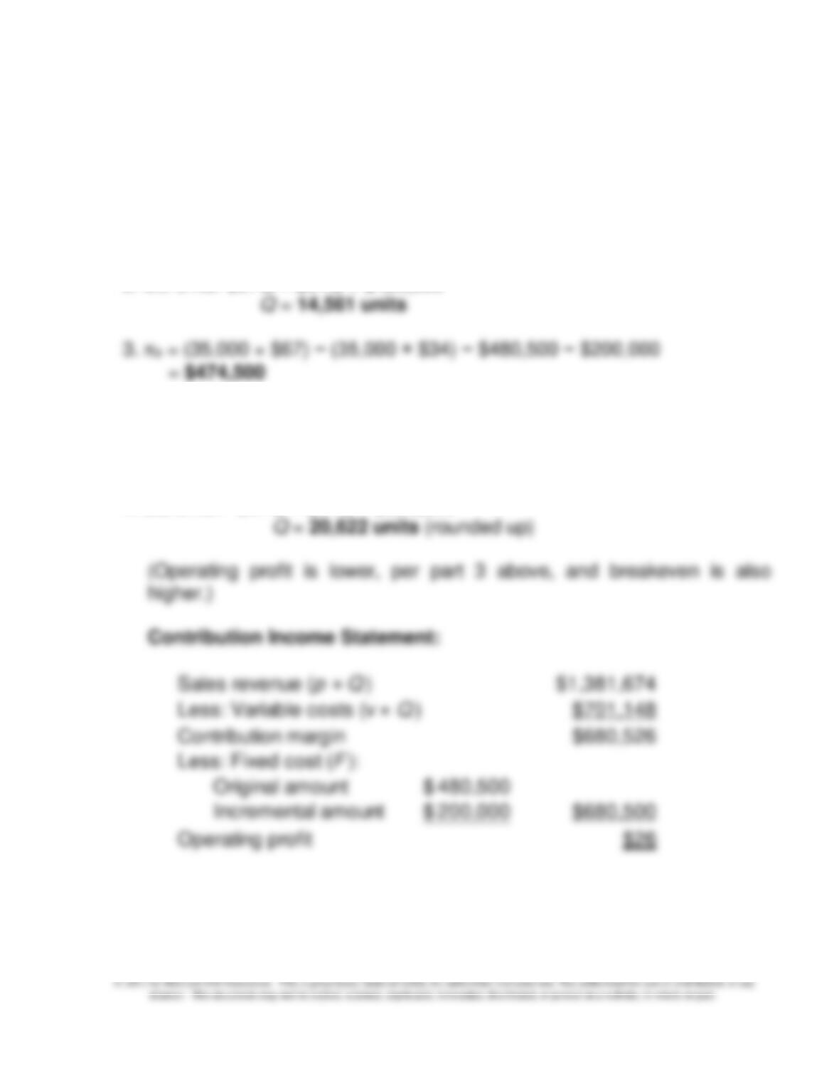
= (30,000 × $67) − (30,000 × $34) − $480,500
= $509,500
2. BE units: $67Q = $34Q + $480,500
(Operating profit falls by $35,000 = ($33 × 5,000) − $200,000, from
$509,500 to $474,500 as a result of the plan to increase sales with
increased advertising.)
4. BE units: $67Q = $34Q + $680,500
(the slight difference between the indicated operating profit,
$26, and zero is due to rounding up the breakeven point to the
nearest whole number, 20,622 units)
Chapter 9 – Short-Term Profit Planning: Cost-Volume-Profit (CVP) Analysis
9-6
Slight difference in the above answers is due to
rounding on sales volume, Q. The primary point,
however, is that a given percentage change in fixed
cost leads to an equivalent percentage change in the
breakeven point. (This can be confirmed precisely if the
above breakeven volumes were not rounded.)
9-21 (Continued)
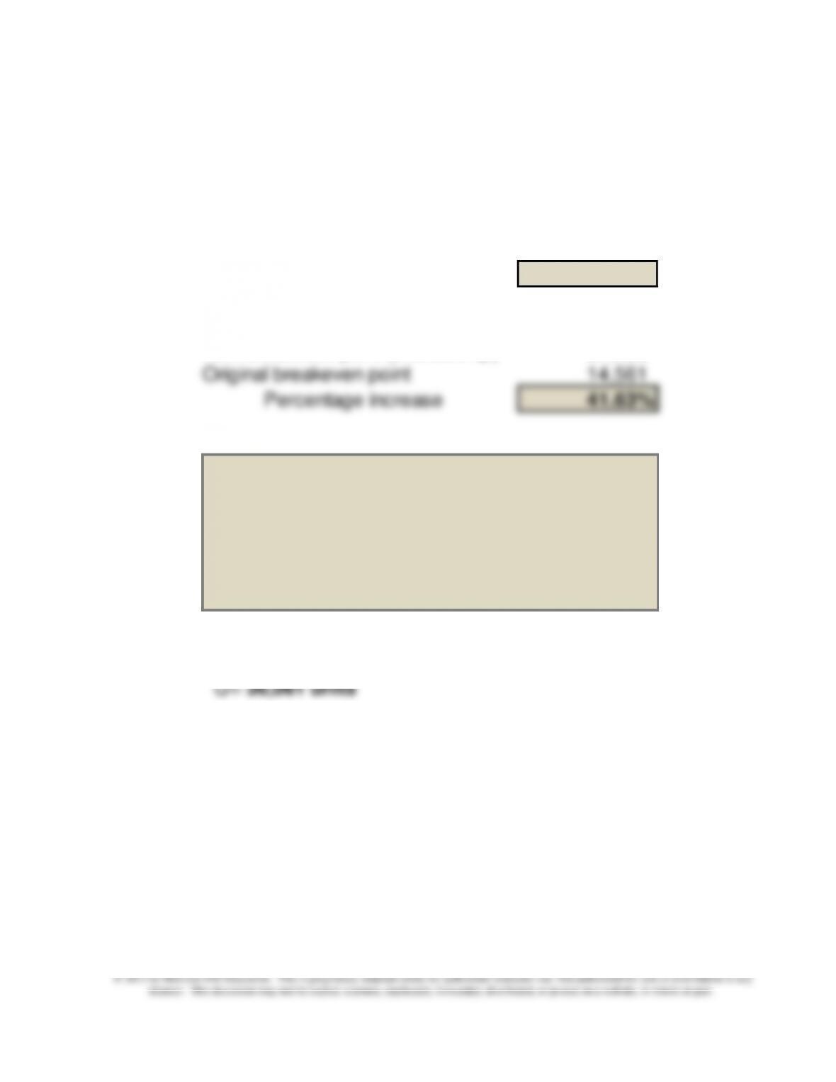
Percentage increase in fixed cost (F):
New level of fixed cost $680,500
Original level of fixed cost $480,500
Percentage increase 41.62%
Percentage increase in breakeven point:
New breakeven point (rounded up) 20,622
Original breakeven point
14,561
Percentage increase 41.63%
5. $509,500 = $67Q − $34Q − $680,500
(To justify the advertising plan, sales would have to rise to at least 36,061
units, somewhat above the projected level of 35,000 units.)
Chapter 9 – Short-Term Profit Planning: Cost-Volume-Profit (CVP) Analysis
9-7
9-22 Margin of Safety (MOS) (20 min)
1. First, calculate the breakeven point, using the contribution margin ratio
(CMR), as follows:
CMR = $227,500 ÷ $650,000 = 0.35
Breakeven in dollars = $105,000 ÷ 0.35 = $300,000
Therefore:
2. The MOS and related MOS ratio (or, percentage) are rough measures of
operating risk. They indicate the amount by which sales could fall before
losses are incurred.
3. If sales fall to $500,000, the breakeven point will remain the same, but the
MOS will change:
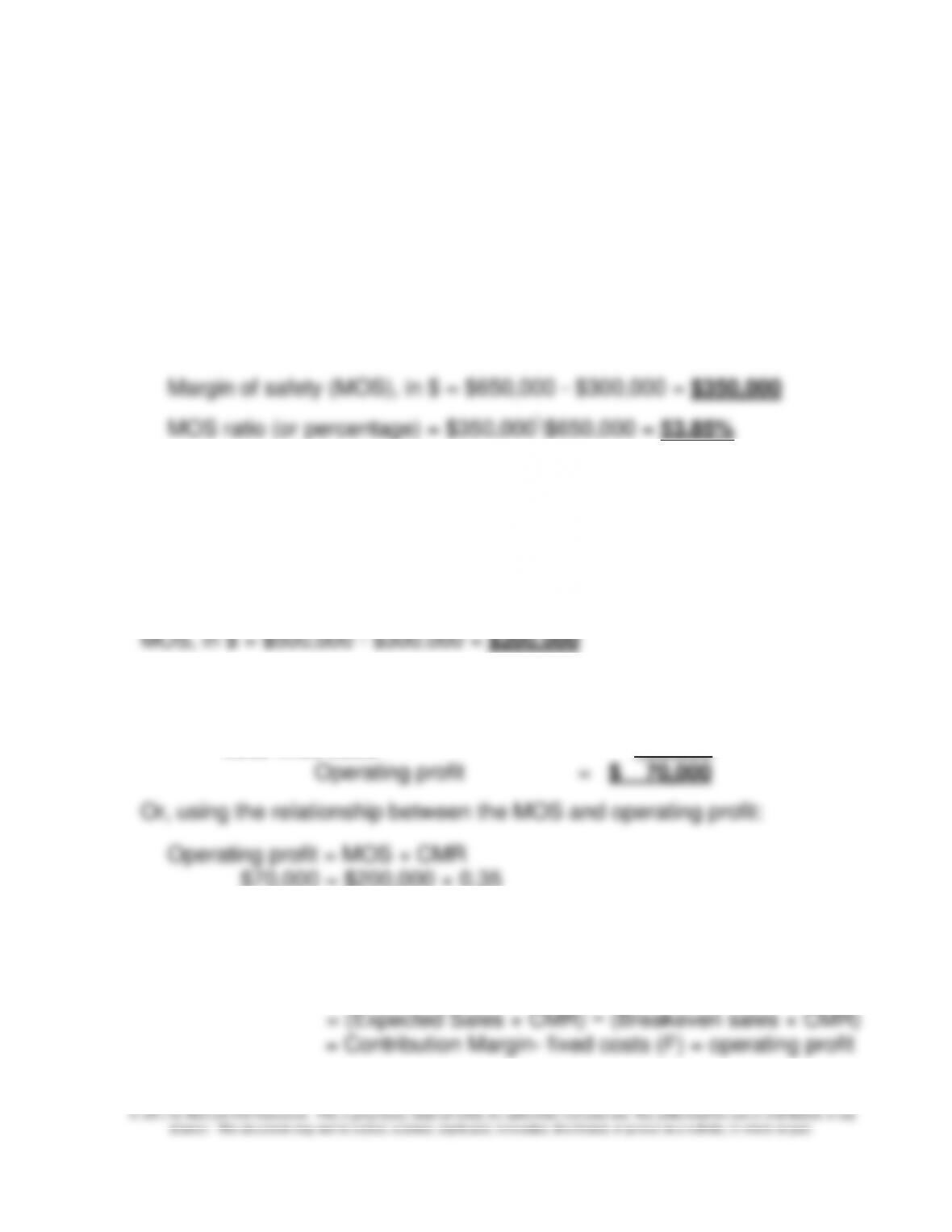
MOS, in $ = $500,000 – $300,000 = $200,000
Operating profit:
Contribution margin = $500,000 × 0.35 = $175,000
Less fixed costs 105,000
Why this works:
Operating profit = MOS × CMR
= (Expected Sales − Breakeven) × CMR
Chapter 9 – Short-Term Profit Planning: Cost-Volume-Profit (CVP) Analysis
9-8
9-22 (Continued)
(Note: by definition, breakeven in sales dollars × CMR = fixed costs; i.e., at the
breakeven point there is just enough contribution margin generated to cover
total fixed costs)
9-23 The Role of Income Taxes (20 min)
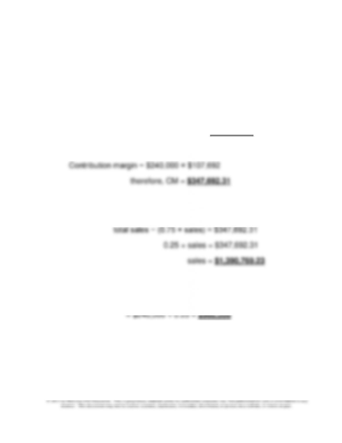
1. Pre-tax income = $70,000 ÷ (1 − 0.35) = $107,692.31
2. Contribution margin − fixed cost = before tax profit
3. total sales – total variable cost = total contribution margin
total sales – (variable cost ratio × sales) = $347,692.31
4. Contribution margin ratio (CMR) = $347,692.31 ÷ $1,390,769.31 = 0.25
Breakeven point = fixed costs ÷ CMR
Chapter 9 – Short-Term Profit Planning: Cost-Volume-Profit (CVP) Analysis
9-9
9-24 CVP Analysis with Taxes (20-25 min)
1. BE units = F + πB = $75,000 + 0 = 18,750 units
(p – v) $10 − $6
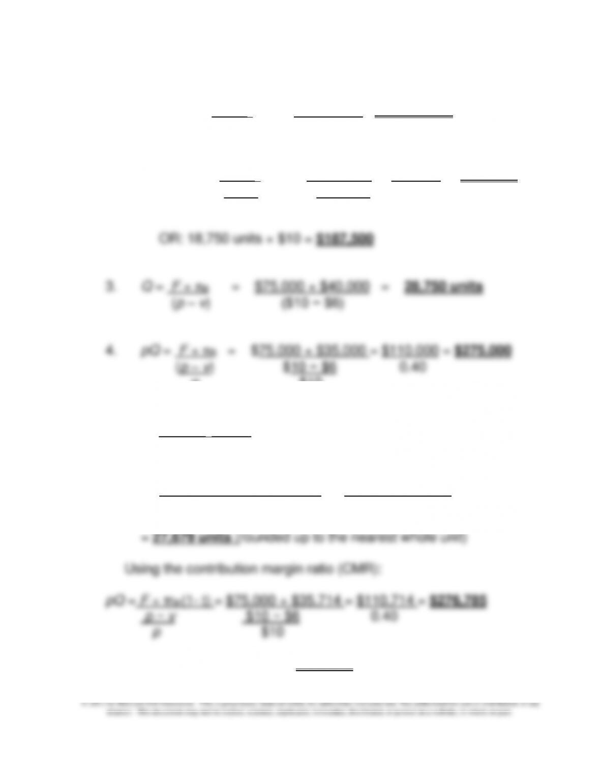
2. BE dollars = F + πB = $75,000 + 0 = $75,000 = $187,500
(p – v) $10 − $6 0.40
p $10
p $10
5. Q = F + πA/(1 − t)
(p – v)
Q = $75,000 + $25,000/(1 − 0.3) = $75,000 + $35,714
$10 − $6 $4
OR: 27,679 units × $10/unit = $276,790 (difference due to rounding)
Chapter 9 – Short-Term Profit Planning: Cost-Volume-Profit (CVP) Analysis
9-10
9-25 Cost Planning; Machine Replacement (30 min)
1.
Machine A Machine B
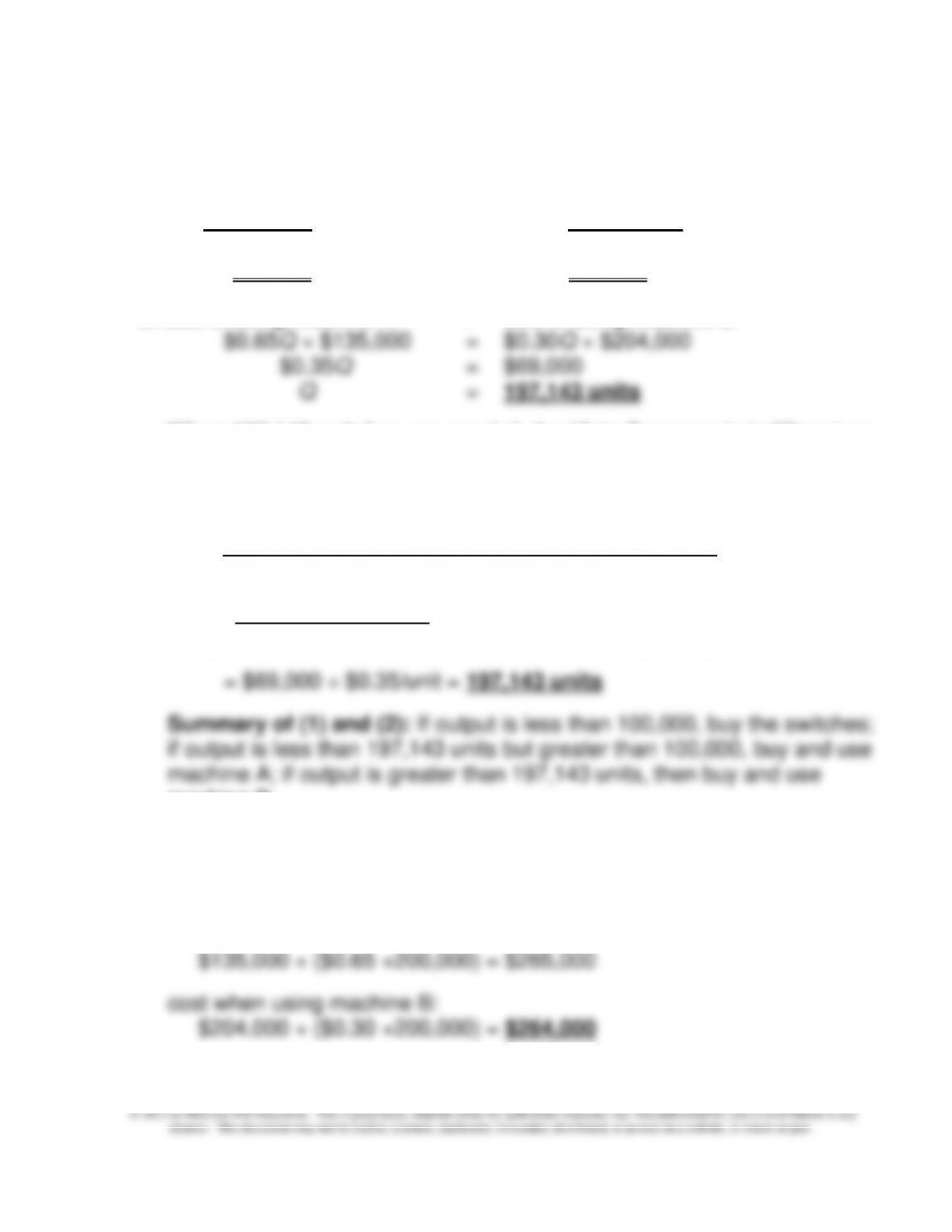
$2Q = $0.65Q + $135,000 $2Q = $0.3Q + $204,000
Q = 100,000 Q = 120,000
2. cost of using Machine A = cost of using Machine B
When 197,143 switches are needed, the Vista Company is indifferent as
to which machine to use.
An alternative way to determine the indifference point is:
Fixed cost of Machine A − Fixed Cost of Machine B
Unit variable cost of A − Unit variable cost of B
$204,000 − $135,000
$0.65 − $0.30
machine B.
3.
cost when purchasing from outside supplier:
$2 × 200,000 = $400,000
cost when using machine A:
Chapter 9 – Short-Term Profit Planning: Cost-Volume-Profit (CVP) Analysis
9-11
9-25 (continued-1)
4. Recommendation to management:
Considerations regarding outsourcing (rather than making internally):
what is the reliability of the existing supplier? Likely price increases in the
future from this supplier? What is the reliability of the external supplier
(delivery time, etc.)? As we’ve seen with supply disruptions in Japan
subsequent to the 2011 tsunami/earthquake in Japan, it may make
Considerations regarding insourcing (rather than purchasing
externally from the current supplier): is sufficient capital (to purchase and
install machinery) available? Are there any training-related costs to be
borne? The decision to insource increases the operating leverage of the
company, which in turn increases the business (or operating) risk of the
company. Therefore, what is the long-term upside potential for increases
in sales—if large, then perhaps a move to a greater level of fixed costs
makes sense. What are anticipated year-to-year fluctuations in
sales/demand for the component in question? If these are significant,
then perhaps lower operating leverage is more advantageous. Finally, by
locking the company into a certain technology, does this decrease
flexibility (for future investments in alternative technologies, as an
example)?
The basic point to make to students is that choice of cost structure both
reflects and influences a company’s strategy. This elevates the
Chapter 9 – Short-Term Profit Planning: Cost-Volume-Profit (CVP) Analysis
9-12
9-26 Degree of Operating Leverage (DOL) (20 min)
1. DOL = contribution margin÷ operating profit
A’s DOL = $50,000 ÷ $35,000 = 1.43
B’s DOL = $70,000 ÷ $30,000 = 2.33
If sales increase, company B will benefit more. Company B has a higher
proportion of fixed costs in relation to variable costs; therefore it has a
higher operating leverage than does Company A. The degree of
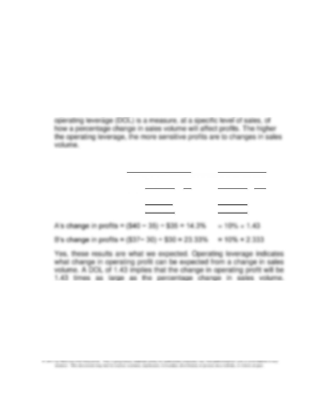
2. COMPANY A COMPANY B
Amount % Amount %
Sales $110,000 100 $110,000 100
Less variable costs 55,000 50 33,000 30
Contribution margin $ 55,000 50 $ 77,000 70
Less fixed costs 15,000 40,000
Operating income $ 40,000 $ 37,000
Therefore, if sales volume increased by 10%, operating profit should
increase by 14.3%. This is precisely what happened. The same logic
applies to Company B.
Chapter 9 – Short-Term Profit Planning: Cost-Volume-Profit (CVP) Analysis
9-13
9-26 (Continued)
3. Further interpretation of DOL—in what sense is DOL a measure of risk?
As indicated by the above responses, DOL measures how sensitive
operating profits are to changes in sales volume. If DOL is high, then
even small (%) changes in sales will lead to large (%) changes in
operating income. It is this magnification process that captures what is
called business or operating risk (as compared, for example, to financial
Finally, we note that DOL can be defined as: % change in operating
income/% change in sales (i.e., the percentage change in operating
income for each percentage change in sales volume from point Q).
Chapter 9 – Short-Term Profit Planning: Cost-Volume-Profit (CVP) Analysis
9-14
9-27 Cost Planning: The Cost of an MBA; Time Value of Money (10 min)
Using the present value factor (4.212) for an annuity for five years at 6% shows
that the present value of $23,742 per year is $100,000 ($100,000 ÷ 4.212); this
means that for the student a current payment (at one point in time in this
simplified example) of $100,000 is equivalent to receiving a benefit of $23,742
Note that the cost of the program includes the foregone pre-MBA salary, and
for students at prestigious programs like School B, the pre-MBA salaries are
relatively high. So the increase in salary post-MBA does not show the degree
of “bump” that is seen in other schools. Also, the calculation above does not
reflect the opportunity that might attract a new MBA to a company, apart from
the pay offer. For example, BusinessWeek provides a listing of its Top-50
Employers, based on surveys of students, college placement personnel, and
the employers themselves. As of September 2008, the Big-4 public accounting
firms, Goldman Sachs, Google, Marriott, Lockheed Martin, IBM and
JPMorgan/Chase lead the list.
Another Business Week survey shows the cost and increase in pay for 20 well–
know U.S. universities. Brigham Young University is shown as the top value
with a high ratio of pay increase to cost.
A Wall Street Journal ranking of the return on investment for top executive
MBA programs, based on tuition costs and projected salary, shows surprising
results, among them that the top five programs are at public Universities; the
highest-ranked program, Texas A&M University, produced a 243% return on
investment.
Source: “The High Price of Admission,” BusinessWeek, October 23, 2006, p.
60. Also: “Fifty Employers with the Right Stuff,” BusinessWeek, September 15,
2008, p. 39; Alina Dizik, “Ranking the Returns on Executive MBAs,” The Wall
Street Journal, December 10, 2008, p D1.
Chapter 9 – Short-Term Profit Planning: Cost-Volume-Profit (CVP) Analysis
9-15
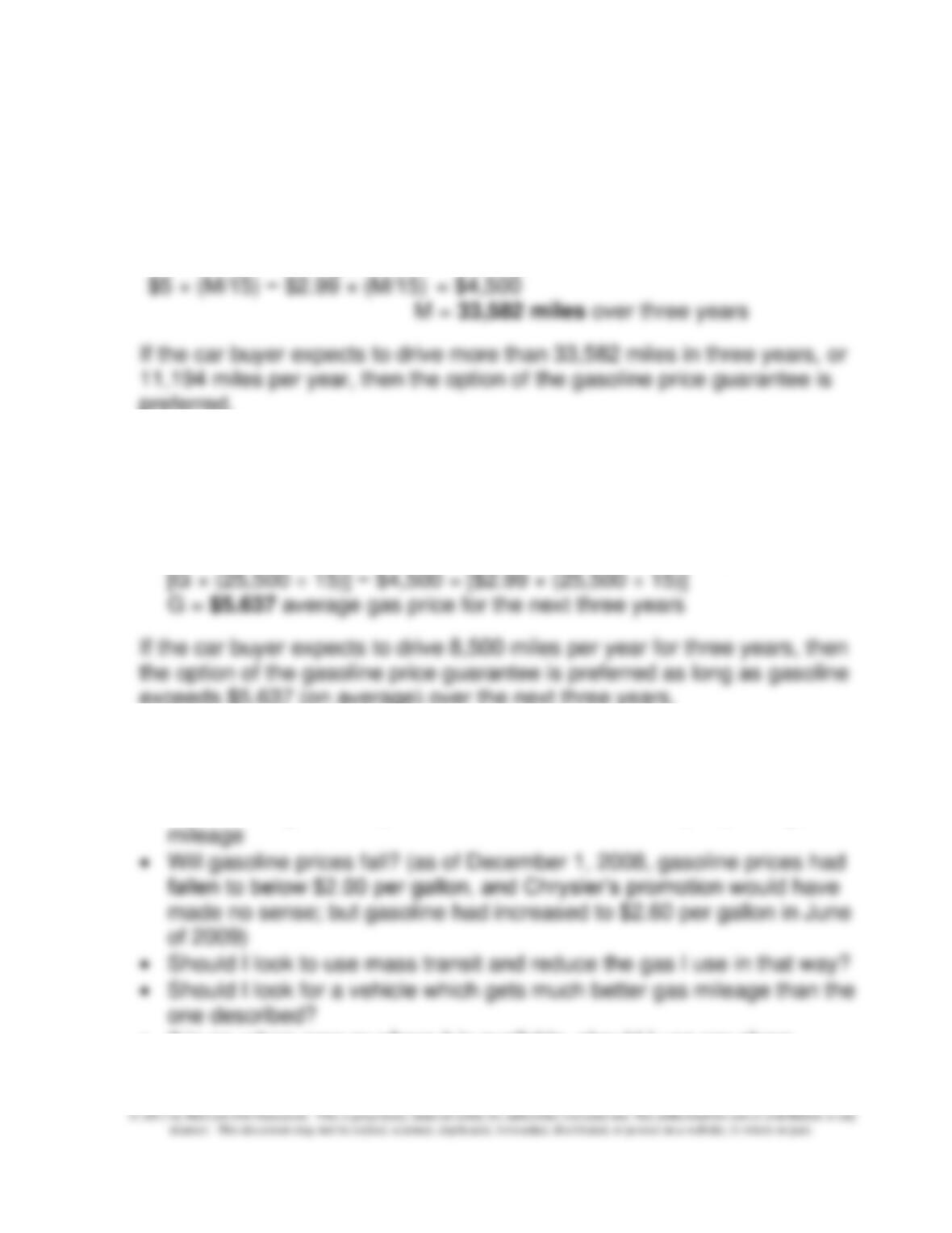
9-28 Cost Planning; Gasoline Prices (20-25 min)
1. Solve for the indifference point in miles (M) where 15 is the mpg, and $2.99
is the guarantee price and $5.00 is the expected price:
Savings for the guarantee = Savings for the discount
preferred.
2. Solve for the indifference point in gasoline price (G) where 15 is the mpg,
and $2.99 is the guaranteed price and 8,500 is the expected annual mileage
(8,500 × 3 years = 25,500 miles for three years):
Total cost without the guarantee = Total cost with guaranteed gas price
exceeds $5.637 (on average) over the next three years.
3. Some important decision factors include:
• Do I need a new car, or should I save the money by fixing up my present
car, including a tune up and new tires which could help improve gas
• If in an urban area or where it is available, should I use car-share
programs?