Chapter 9 – Short-Term Profit Planning: Cost-Volume-Profit (CVP) Analysis
9-74
9-49 (continued-4)
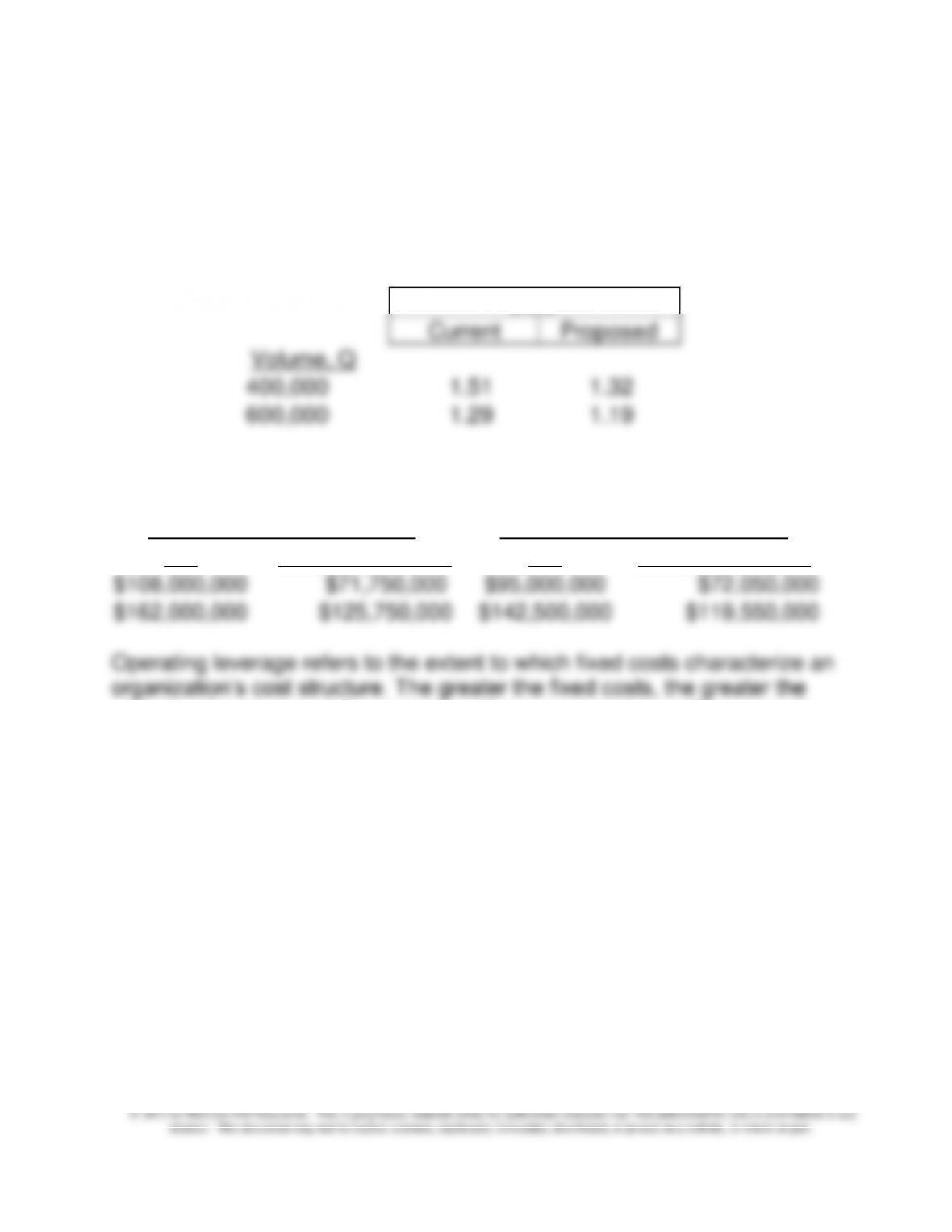
5. Calculation and interpretation of degree of operating leverage (DOL) under
each decision alternative at Q = 400,000 units and at Q = 600,000 units.
DOL, at any volume level, Q = CM ÷ Operating Income
Backup information for DOL calculations:
DOL Components (Current)
DOL Components (Proposed)
CM
Operating Income
CM
Operating Income
$108,000,000
$71,750,000
$95,000,000
$72,050,000
$162,000,000
$125,750,000
$142,500,000
$119,550,000
Operating leverage refers to the extent to which fixed costs characterize an
organization’s cost structure. The greater the fixed costs, the greater the
operating leverage and the more sensitive or responsive profits are to changes
in sales volume.
DOL
Chapter 9 – Short-Term Profit Planning: Cost-Volume-Profit (CVP) Analysis
9-75
9-49 (continued-5)
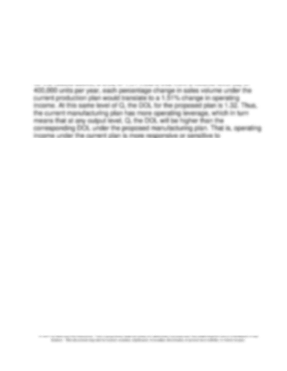
A measure of the extent to which profits vary in response to changes in sales
volume is the degree of operating leverage (DOL). DOL represents the
percentage change in operating profit per percentage change in sales. Thus,
changes in sales volume. Relative to the proposed plan, the current plan would
generate greater percentage reductions in operating income if sales volume
declines, but greater percentage increases in operating income in response to
increases in sales volume. In this sense, the operating risk associated with the
current plan is greater than the operating risk associated with the proposed
plan.
Chapter 9 – Short-Term Profit Planning: Cost-Volume-Profit (CVP) Analysis
9-76
Problem 9-50: CVP Analysis; Sustainability; Uncertainty; Decision Tables
(60-75 min)
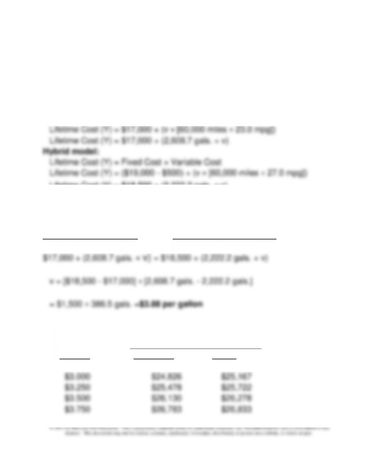
1. Lifetime cost functions: let Y = lifetime cost, and v = cost per gallon of
gas
Regular model:
Lifetime Cost (Y) = Fixed Cost + Variable Cost
Lifetime Cost (Y) = $17,000 + (v × [60,000 miles ÷ 23.0 mpg])
Lifetime Cost (Y) = $17,000 + (2,608.7 gals. × v)
Hybrid model:
Lifetime Cost (Y) = Fixed Cost + Variable Cost
Lifetime Cost (Y) = ($19,000 – $500) + (v × [60,000 miles ÷ 27.0 mpg])
Lifetime Cost (Y) = $18,500 + (2,222.2 gals. × v)
2. Breakeven gas price (point of cost indifference): let “v” = breakeven price per
gallon
Lifetime Cost—Gas Model = Lifetime Cost—Hybrid Model
$17,000 + (2,608.7 gals. × v) = $18,500 + (2,222.2 gals. × v)
v = [$18,500 – $17,000] ÷ [2,608.7 gals. – 2,222.2 gals.]
= $1,500 ÷ 386.5 gals. =$3.88 per gallon
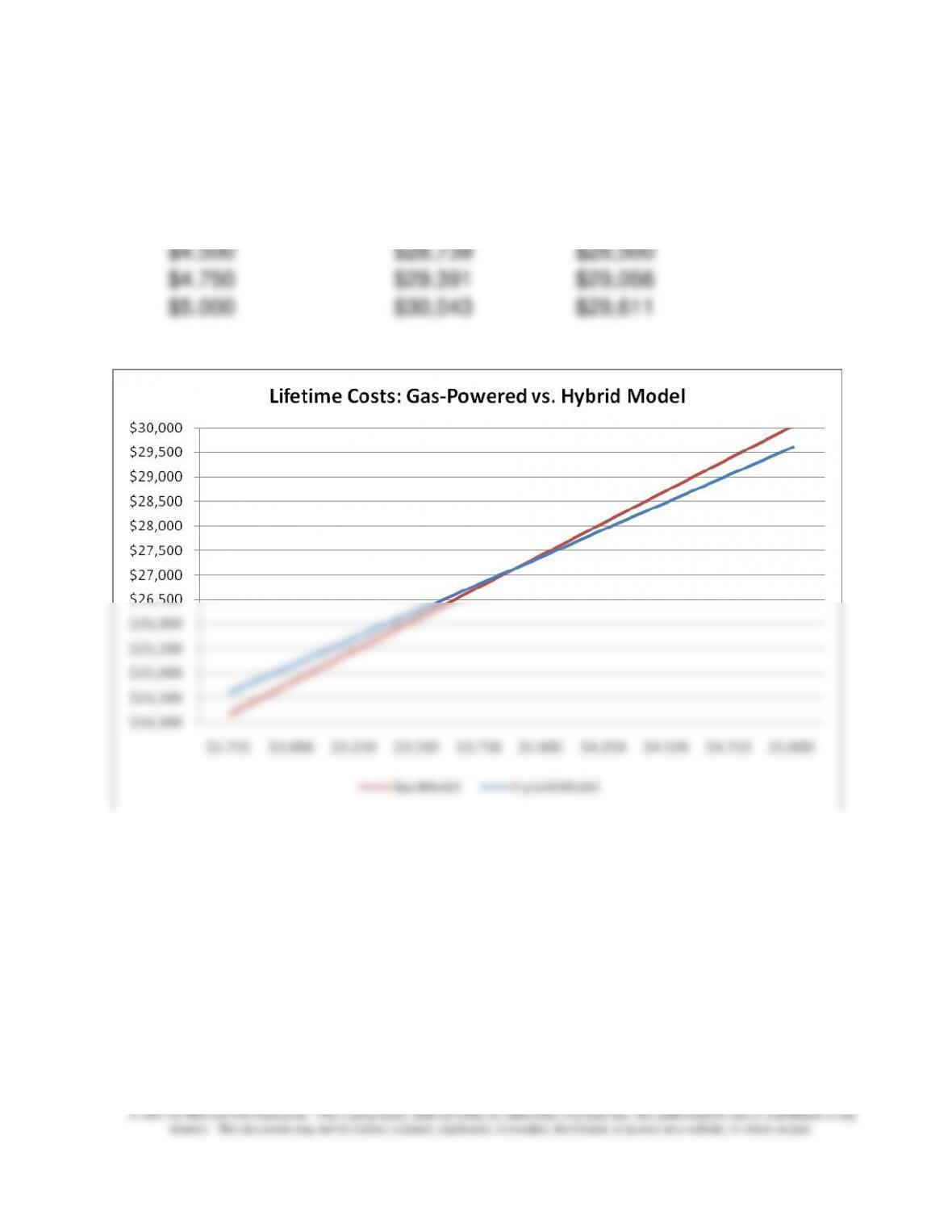
3. Graph of Lifetime Cost Function—Regular and Hybrid Models
X (price
Lifetime Cost
per gal.)
Gas Model
Hybrid
$2.750
$24,174
$24,611
$3.000
$24,826
$25,167
$3.250
$25,478
$25,722
$3.500
$26,130
$26,278
$3.750
$26,783
$26,833
Chapter 9 – Short-Term Profit Planning: Cost-Volume-Profit (CVP) Analysis
9-77
9-50 (Continued-1)
$4.000
$27,435
$27,389
$4.250
$28,087
$27,944
$4.500
$28,739
$28,500
$4.750
$29,391
$29,056
$5.000
$30,043
$29,611
Based on the above analysis and graph, we see that for these two
alternatives (gas-powered vs. hybrid model), and 60,000 miles total usage
over a four-year period, the lifetime costs are close, that is, they are
insensitive to the predicted cost of gas per gallon.
Chapter 9 – Short-Term Profit Planning: Cost-Volume-Profit (CVP) Analysis
9-78
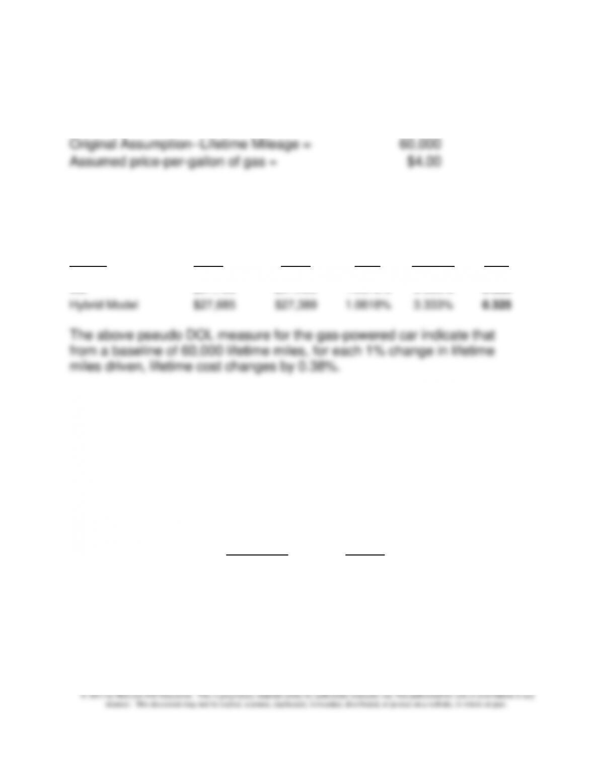
4. Pseudo degree of operating leverage (DOL) measure
Alternative Lifetime Mileage Assumption =
62,000
Original Assumption—Lifetime Mileage =
60,000
Assumed price-per–gallon of gas =
$4.00
9-50 (Continued-2)
Lifetime Cost
Lifetime Cost
%
Option
@ 62,000
miles
@ 60,000
miles
Change
Cost
% Change
Mileage
Pseudo
DOL
Gas Powered
Car
$27,783
$27,435
1.2678%
3.333%
0.380
Hybrid Model
$27,685
$27,389
1.0818%
3.333%
0.325
The above pseudo DOL measure for the gas-powered car indicate that
from a baseline of 60,000 lifetime miles, for each 1% change in lifetime
miles driven, lifetime cost changes by 0.38%.
The relevant measure for the hybrid, from this base, is 0.325%. What this
tells us is that for this particular example, lifetime cost for both decision
alternatives is approximately equally sensitive to changes in lifetime miles
driven.
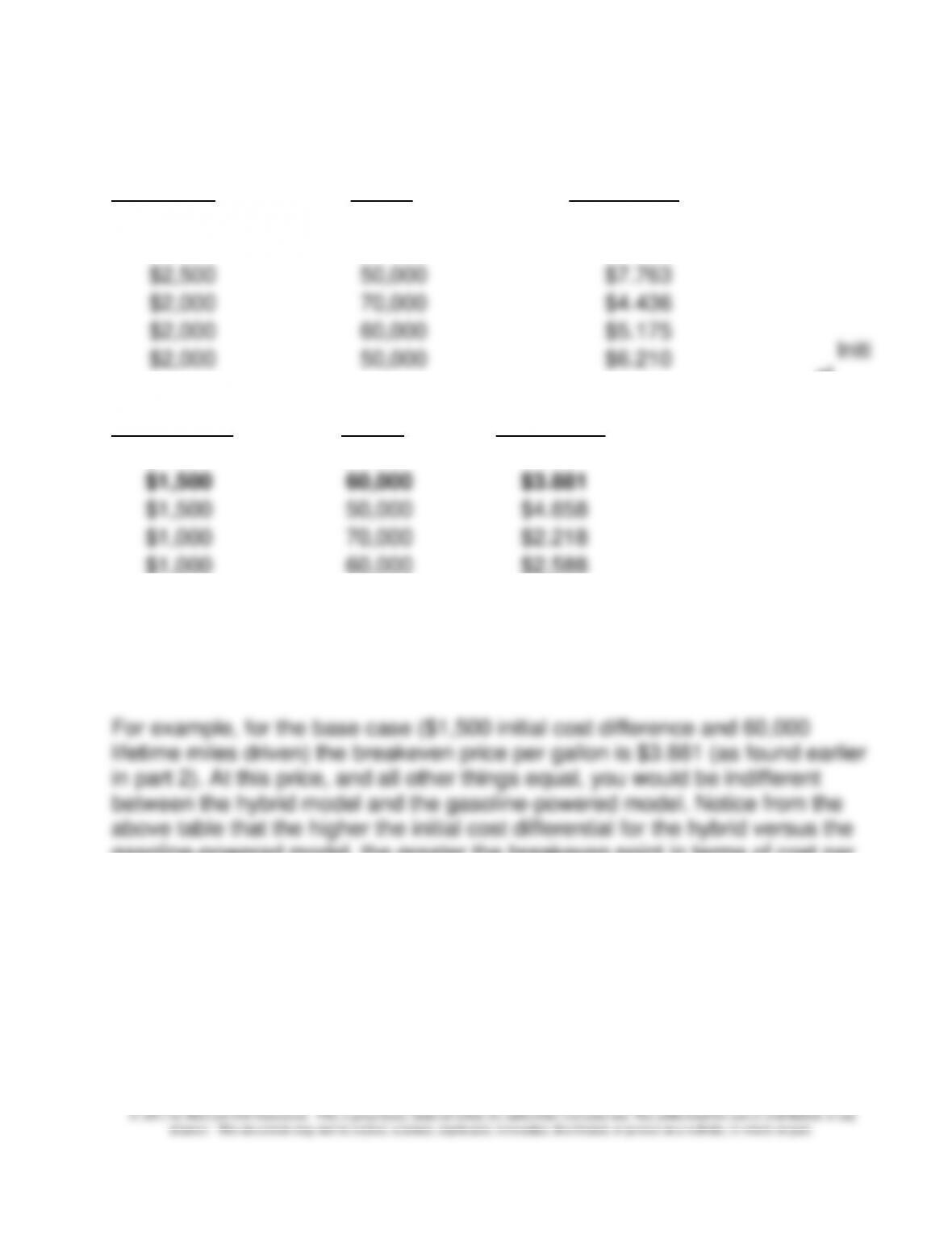
5. Decision Table—Break-even gas price as a function of different
combinations of initial cost differential (Hybrid cost [net of rebate] −
Cost of gasoline-powered model) and lifetime miles driven
Initial Cost
Difference
Lifetime Miles
Driven
$2,500
70,000
$2,000
60,000
$1,500
50,000
$1,000
$500
Chapter 9 – Short-Term Profit Planning: Cost-Volume-Profit (CVP) Analysis
9-79
9-50
(cont
inued
-3)
$2,500
50,000
$7.763
$2,000
70,000
$4.436
$2,000
60,000
$5.175
al
Cost Lifetime Miles Gas Price
Differential Driven (per gallon)
$1,500
70,000
$3.327
$1,500
60,000
$3.881
$1,500
50,000
$4.658
$1,000
70,000
$2.218
$1,000
60,000
$2.588
$1,000
50,000
$3.105
$500
70,000
$1.109
$500
60,000
$1.294
$500
50,000
$1.553
gasoline-powered model, the greater the breakeven point in terms of cost per
gallon of fuel. You also notice that the breakeven gas price is inversely related
to lifetime miles driven. While both conclusions seem intuitively appealing, the
advantage of the decision table is the structured way in which it allows you to
deal quantitatively with uncertainty surrounding the financial consequence of
your decision choice.
Initial Cost
Differential
Lifetime Miles
Driven
Breakeven Gas Price
(per gallon)
$2,500
70,000
$5.545
$2,500
60,000
$6.469
$2,000
50,000
$6.210
Chapter 9 – Short-Term Profit Planning: Cost-Volume-Profit (CVP) Analysis
9-80
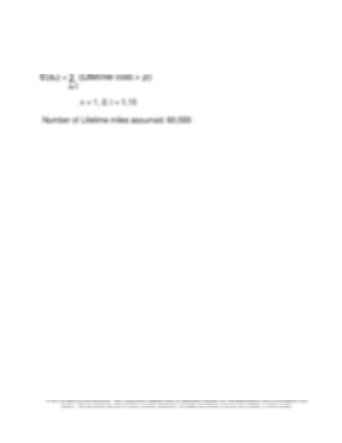
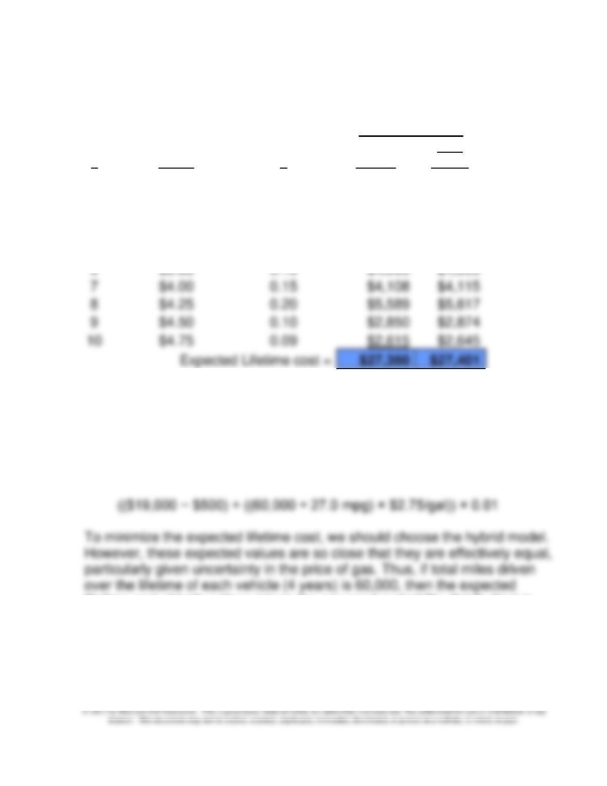
6. Expected value calculations:
10
Chapter 9 – Short-Term Profit Planning: Cost-Volume-Profit (CVP) Analysis
9-81
9-50 (continued-4)
Action (Decision)
i
Event
p
Hybrid
Gas
Model
1
$2.75
0.01
$246
$242
2
$3.00
0.05
$1,258
$1,241
3
$3.25
0.05
$1,286
$1,274
4
$3.50
0.05
$1,314
$1,307
5
$3.75
0.15
$4,025
$4,017
6
$3.88
0.15
$4,069
$4,069
7
$4.00
0.15
$4,108
$4,115
8
$4.25
0.20
$5,589
$5,617
9
$4.50
0.10
$2,850
$2,874
10
$4.75
0.09
$2,615
$2,645
Expected Lifetime cost =
$27,360
$27,401
Lifetime cost = initial cost outlay (F) + variable (gas) cost over four-year
period
Example: for the hybrid model, if the probability of gas selling at $2.75/gallon
is 0.01, then the appropriate amount is cost component for
calculating expected lifetime cost is:
lifetime cost of both actions (given the assumed probability distribution) is
approximately equal.
Finally, note that basing the decision solely on expected value (in the
present case, cost) ignores the risk preferences (utility function) of the
Chapter 9 – Short-Term Profit Planning: Cost-Volume-Profit (CVP) Analysis
9-82
decision-maker. The decision table presented above in part 5 can facilitate
this discussion.
9-50 (continued-5)
7. Student answers will likely differ. Below are representative considerations.
Qualitative Considerations
a. safety record—does this differ between the two models?
b. reliability—does this differ between the two models? (in some cases, the
reliability of new models is considerably less than the reliability of older,
on total miles driven, its carbon footprint might be larger than it is for a
related gasoline-powered model.
e. relationship between mpg and lifetime miles driven: ignored thus far in the
analysis is the fact that the latter might be a function of the former. Our
analysis has, in fact, assumed that these two variables are unrelated (i.e.,
Chapter 9 – Short-Term Profit Planning: Cost-Volume-Profit (CVP) Analysis
9-83
Additional Quantitative Considerations
a. what is the estimated useful life for each vehicle? (this would be important
if the buyer intended to use the vehicle beyond the four-year planning
horizon)
b. related to the above point, what is the estimated salvage/disposal value of
each vehicle at the end of the four-year decision horizon?
c. related to point b above, what is the estimated salvage value at the end of
(similar to the approach taken in capital budgeting decisions).
f. the given mpg figures are based on some type of average driving (or mix
between city and highway miles driven). Is the anticipated driving behavior
of the purchaser different from this assumed mix so that the use of average
mpg data would not be appropriate? If most of the driving is done in the
city, this is a distinct advantage for the hybrid, since electric propulsion
would be used more frequently in this context. On the other hand, if most
Chapter 9 – Short-Term Profit Planning: Cost-Volume-Profit (CVP) Analysis
9-84
Check Figures: Chapter 9
9-21 1. $509,500; 2. 14,561 units; 3. $474,500; 4. 20,622 units (rounded up); 5. 36,061
units
$2,600
9-30 No check figure.
9-31 No check figure.
9-32 1. Total B/E units = 517.65; 2. Brighter, 207.05882; Cleaner, 310.58824; 3. $465,882
9-33 1.$25,000,000; 2.$51,666,667; 3. Variable cost ratio = 0.7840; B/E = $34,722,222
9-34 2. Required price increase = $101.67
9-35 No check figure.
9-36 No check figure.
9-42 1.($6,500); 2. B/E in total sales dollars = $224,074; 3. Gasoline, $112,037;
Food/beverage = $67,222; Other, $44,815; 4. Profit before tax = $23,500.
9-43 1. B/E = $17,800; 2. Required sales = $30,063 (rounded up); 4. Indifference point =
$14,538 (rounded and in $000s)
9-85
9-44 1. B/E = 3,649 clients per year (rounded up); 2. Expected value = 12,600 clients in
year 1; 4. Probability is approximately 95%; probability of generating at least
plan, and $19 for the proposed plan (note: these differ from zero because the above–
listed breakeven quantities were rounded up to the next whole number)
9-48 1.contribution margin = $11.30 per weekly subscription; contribution margin = $7.30
per monthly subscription; 2. contribution margin ratios: 24.0% (weekly); 38.4%
(monthly); 3. B/E = 37,778 subscriptions (weekly = 7,556; monthly, 30,222); B/E$ =
$929,333 (weekly subscriptions = $355,111; monthly subscriptions = $574,222); 6.
required sales volume = 47,037 units; 7. required sales volume = 66,729 units
9-49 1.unit contribution margins, $270.00 (current) and $237.50 (proposed); B/E = 134,260
(current), and 96,632 (proposed); 2. Indifference point = 409,231 units; 5. DOL at Q =