Chapter 9 – Short-Term Profit Planning: Cost-Volume-Profit (CVP) Analysis
9-46
9-43 CVP Analysis; Commissions; Ethics (50 min)
1. Breakeven dollars (dollars in thousands), Y:
Y = total fixed costs ÷ contribution margin ratio
Y = ($6,120 + $1,890) ÷ (1 − VCGS rate − commissions rate)
Supporting Calculations
Variable cost of goods sold rate (dollars in thousands):
$11,700 ÷ $26,000 = 45%
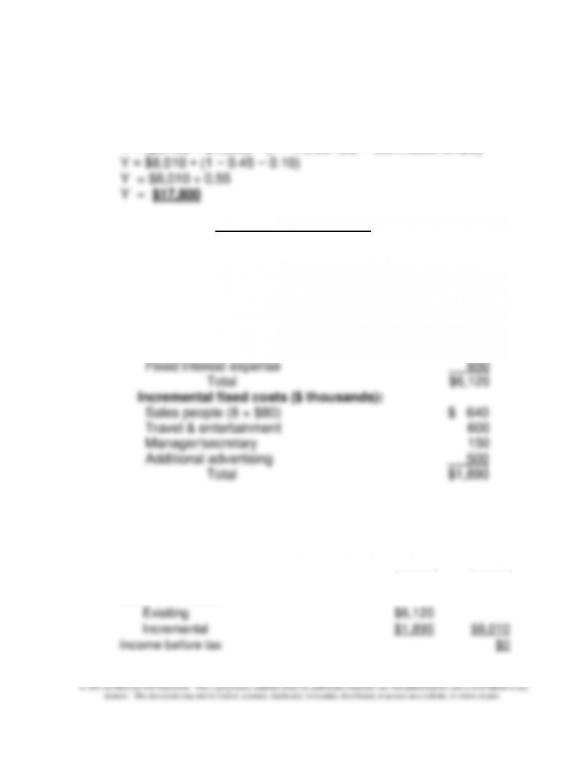
Current fixed costs ($ thousands):
Fixed cost of goods sold $2,870
Fixed advertising cost 750
Fixed administrative cost 1,850
Check:
Sales $17,800
Variable costs:
manufacturing (CGS) $8,010
sales commissions $1,780 $9,790
Contribution margin $8,010
Less: Fixed Costs:
Exisiting $6,120
Incremental $1,890 $8,010
Income before tax $0
Chapter 9 – Short-Term Profit Planning: Cost-Volume-Profit (CVP) Analysis
9-47
9-43(Continued-1)
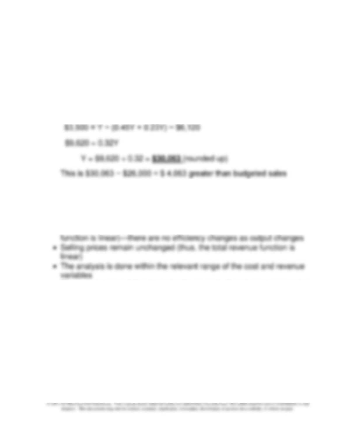
2. Required sales (to maintain current level of pre-tax income, $3,500, while
paying the requested increase in commission):
Let Y = required sales level:
$3,500 = Total sales − total variable costs − total fixed costs
3. The general assumptions underlying breakeven analysis that may limit its
usefulness include the following:
• All costs can be divided into fixed and variable elements.
• Variable costs vary proportionally to volume (thus, the variable cost
• The underlying model is deterministic; as such, the inherent assumption
is that the inputs to the CVP model are known with certainty
4. Let sales at the indifference point be Y (in 000s).
Since the two decision alternatives do not affect the selling price per
unit, we can define the indifference point as the volume level that
results in equal total cost between the two decision alternatives:
Chapter 9 – Short-Term Profit Planning: Cost-Volume-Profit (CVP) Analysis
9-48
9-43 (Continued-2)
Total Cost for Current Agents = Total cost for Our Agents
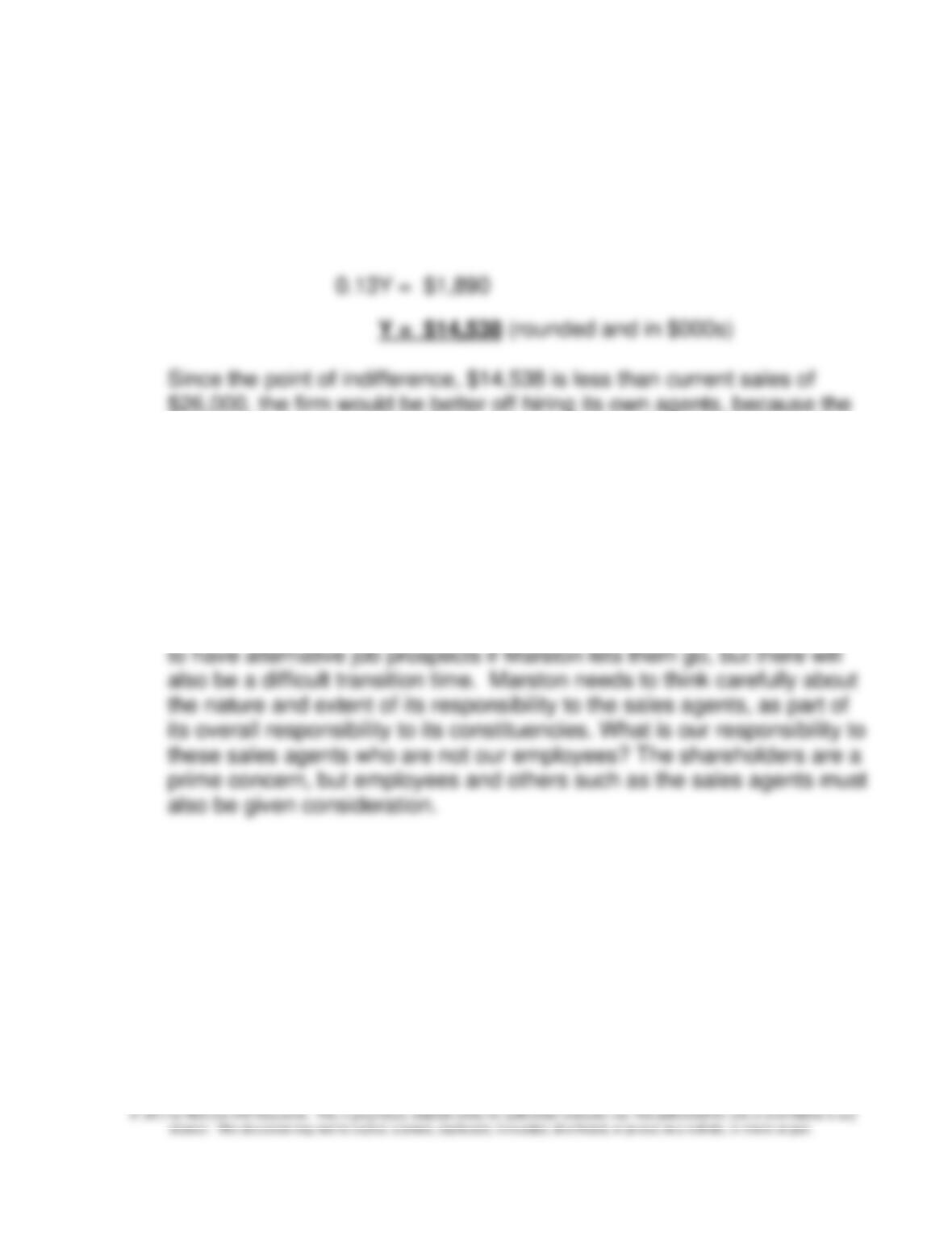
0.45Y + 0.23Y + $6,120 = 0.45Y + $6,120 + $1,890 + 0.10Y
$26,000, the firm would be better off hiring its own agents, because the
relatively low variable cost offsets the relatively high fixed costs of the
new agents when sales are higher than the indifference point.
5. Markowitz should consider the firm’s ethical responsibility to its
shareholders, employees and agents. The new plan would be a savings
for the firm and thus would have an upward effect on stock price and thus
benefit the shareholders. However, the plan would be a blow to the sales
agents, many of whom may be depend on Marston Corporation for a
significant portion (or perhaps all of) their income. The agents are likely
Chapter 9 – Short-Term Profit Planning: Cost-Volume-Profit (CVP) Analysis
9-49
9-44 CVP Analysis; Uncertainty/Sensitivity Analysis (60-75 min)
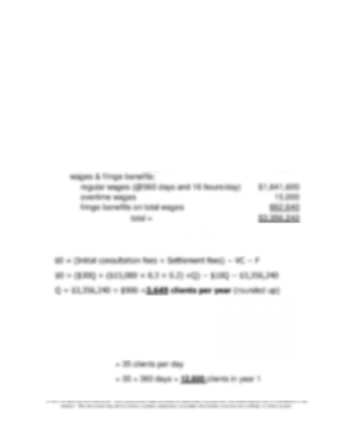
1. In order to break even, during the first year of operations, 3,649 clients
(rounded up) must visit the law office being considered by Don Carson and
his colleagues as calculated below.
Breakeven Calculation:
$0 = Total revenue − variable cost (supplies) − fixed cost (from above)
2. Based on the report of the marketing consultant, the expected number of
new clients during the first year is 12,600 as calculated below. Therefore,
it is entirely feasible for the law office to break even during the first year of
operations as the breakeven point is 3,649 clients (see above).
Expected value = (10 × 0.10) + (20 × 0.30) + (40 × 0.40) + (60 × 0.20)
First-year fixed expenses:
advertising $500,000
rent (6,000 x $48) $288,000
property insurance $22,000
utilities $32,000
malpractice insurance $180,000
depreciation–office equipment
$15,000
wages & fringe benefits:
regular wages (@360 days and 16 hours/day)
$1,641,600
overtime wages 15,000
fringe benefits on total wages 662,640
total = $3,356,240
9-50
9-44 (Continued-1)
Since there is uncertainty in the prediction of the number of clients per
3. Sensitivity Analysis: Sensitivity analysis is used to deal more effectively
with uncertainty or risk. Sensitivity analysis is a “what-if” type of analysis
used to determine the outcomes if any parameters change from the initial
assumptions. For example, revenues or costs could be changed from the
initial assumptions and a new break-even sales volume calculated.
The availability of spreadsheet software has made it very quick and easy
to compute the impact of changing one or more assumptions in a
financial model. At least three factors that make sensitivity analysis
prevalent in decision making include the following:
• As the business environment is becoming more dynamic and
competitive, sensitivity analysis provides management with an
understanding of the impact of changes in the environment. The
clients). Carson can enhance this analysis by using standard
deviations to measure the dispersion of the distributions, as a
means to get at the degree of uncertainty–higher standard
deviations for greater uncertainty.
Chapter 9 – Short-Term Profit Planning: Cost-Volume-Profit (CVP) Analysis
b. probability that the firm will generate at least $3,235,760 of incremental operating
income in year one (from new-client acquisitions):
standard deviation of operating income = $5,000,000 (given)
target profit level = $3,235,760 (given)
expected values:
9-44 (Continued-2)
4. Basic simulation analysis using the NORMDIST function in Excel:
a. probability that the firm will at least breakeven, given normally distributed operating
income and a standard deviation of $5,000,000, is ~ 95%:
Operating Income Information
standard deviation of op. income = $5,000,000 (given)
target pre-tax profit level = $0 (given)
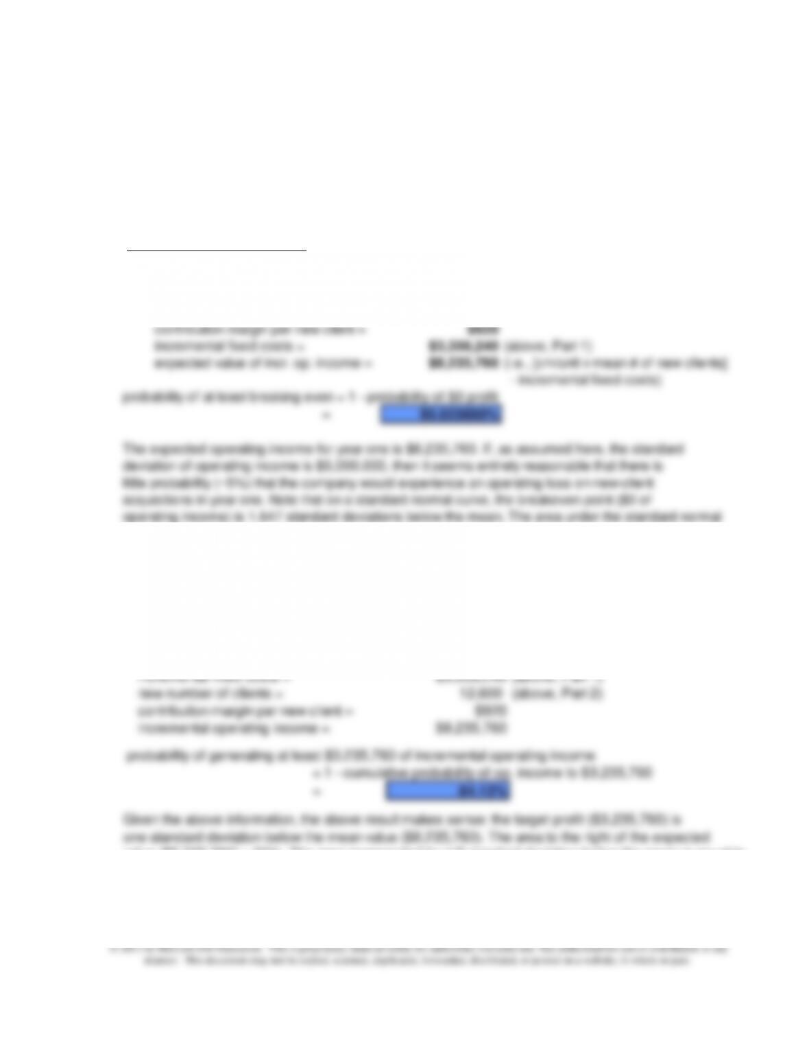
mean (expected) value:
mean expected # new clients = 12,600 (above, Part 2)
contribution margin per new client = $920
incremental fixed costs = $3,356,240 (above, Part 1)
expected value of incr. op. income = $8,235,760 (i.e., [cm/unit x mean # of new clients]
– incremental fixed costs)
probability of at least breaking even = 1 – probability of $0 profit
= 95.023660%
The expected operating income for year one is $8,235,760. If, as assumed here, the standard
deviation of operating income is $5,000,000, then it seems entirely reasonable that there is
little probability (~5%) that the company would experience an operating loss on new-client
acquisitions in year one. Note that on a standard normal curve, the breakeven point ($0 of
operating income) is 1.647 standard deviations below the mean. The area under the standard normal
curve from -1.647 standard deviations to the mean is approximately 45%. Thus, the area from
-1.647 standard deviations below the mean to positive infinity is approximately 95%.
Chapter 9 – Short-Term Profit Planning: Cost-Volume-Profit (CVP) Analysis
9-44 (Continued-3)
c. Given a standard deviation of operating income of $5,000,000 and an expected value of 12,600
new clients in year one. What is the probability of generating incremental operating income of at
least $8,235,760?
standard deviation of operating income = $5,000,000 (given)
target profit level = $8,235,760 (given)
expected values:
incremental fixed costs = $3,356,240 (above, Part 1)
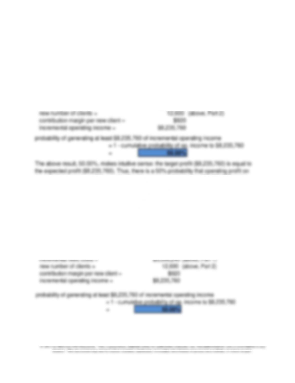
new number of clients = 12,600 (above, Part 2)
contribution margin per new client = $920
incremental operating income = $8,235,760
probability of generating at least $8,235,760 of incremental operating income
= 1 – cumulative probability of op. income to $8,235,760
= 50.00%
The above result, 50.00%, makes intuitive sense: the target profit ($8,235,760) is equal to
the expected profit ($8,235,760). Thus, there is a 50% probability that operating profit on
new clients in year one will be greater than the mean predicted value ($8,235,760) and a
50% probability that operating profit will be less than the mean value. This conclusion derives
from the basic interpretation of a standard normal curve.
d. Given a standard deviation of operating income of $2,500,000 and an expected value of 12,600
new clients in year one, what is the probability of generating incremental operating income of at
least $8,235,760?
standard deviation of operating income = $2,500,000 (given)
target profit level = $8,235,760 (given)
expected values:
incremental fixed costs = $3,356,240 (above, Part 1)
new number of clients = 12,600 (above, Part 2)
contribution margin per new client = $920
incremental operating income = $8,235,760
probability of generating at least $8,235,760 of incremental operating income
Chapter 9 – Short-Term Profit Planning: Cost-Volume-Profit (CVP) Analysis
9-53
9-44 (Continued-4)
What the above result shows, in conjunction with the result from part (c) above, is that if
operating incomes are normally distributed around the mean, then the probabilityof generating
an operating income of at least the mean value is unaffected. Note, however, that the size of
the standard deviation of operating income does affect the size of the confidence interval
around a given targeted value. Note, too, that for a given standardard deviation of
operating income, a change in the standard deviation of operating incomes would affect the
probability of generating a given targeted level of operating income. For example, assume a
targeted operating income of $10,000,000. Given the assumptions in ( c) above, the probability
of generating at least this income is 36.21%; under the situation reflected in (d), the probability
drops to 24.02%.
Chapter 9 – Short-Term Profit Planning: Cost-Volume-Profit (CVP) Analysis
9-54
9-45 CVP Analysis; Strategy; Critical Success Factors (50-60 min)
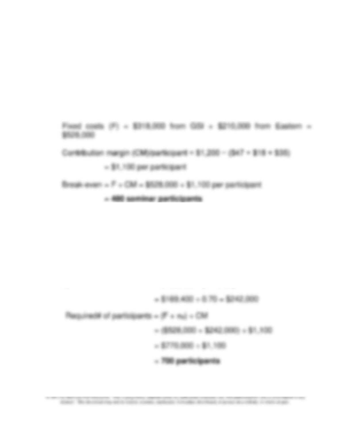
1. a. A total of 480 seminar participants are needed for the joint venture to
break even, calculated as follows:
The break-even number of participants equals the fixed costs divided by
the contribution margin per participant
b. A total of 700 seminar participants are needed for the joint venture to
earn an after-tax profit (πA) of $169,400, calculated as follows.
The target number of participants equals the fixed costs (F) plus the
desired pre-tax profit (πB), divided by the contribution margin per
participant. Note that: πB = πA ÷ (1 − t), where t = the income tax rate.
πB = $169,400 ÷ (1 − 0.30)
Chapter 9 – Short-Term Profit Planning: Cost-Volume-Profit (CVP) Analysis
9-55
9-45 (Continued-1)
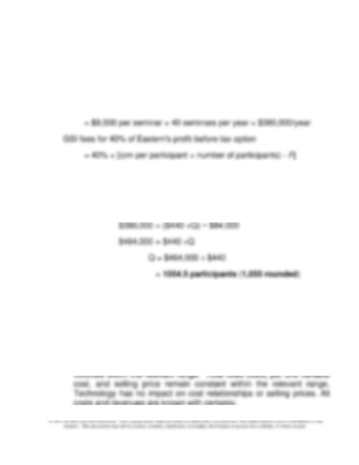
2. A minimum of 1,055 participants is needed in order for GSI to prefer the 40
percent fee option rather than the flat fee, calculated as follows (where Q =
number of seminar participants):
GSI fees for flat fee option
= 0.40 × [($1,100 ×Q) − $210,000)] = ($440 × Q) − $84,000
Pre-tax profit (operating income) would be equal for the two options when
total revenue is equal (since fixed costs of GSI are being ignored for the
present analysis) at the following number of participants, Q.
Therefore, GSI will earn more revenue and prefer the 40 percent option
when the number of participants is 1,055 or higher.
3. Some of the strategic and implementation issues facing GSI in this
decision are the following:
• Are the CVP assumptions satisfied? That is, total costs can be divided
into a fixed component and a component that is variable with respect
to volume. Total costs and total revenues have a linear relationship to
costs and revenues are known with certainty.
Chapter 9 – Short-Term Profit Planning: Cost-Volume-Profit (CVP) Analysis
9-56
9-45 (Continued-2)
• Alternative uses of capacity? Since the Eastern U seminars would
occupy all GSI’s available capacity, GSI should consider whether
there might be more profitable uses for that capacity before making
• Does the collaboration make sense strategically? Are Eastern and
GSI likely to enhance each other’s reputation and to provide operating
synergies and efficiencies that will make the alliance a profitable one?
For example, if the Eastern University’s academic reputation might
suffer from this alliance, then this should be considered in the
decision.
Chapter 9 – Short-Term Profit Planning: Cost-Volume-Profit (CVP) Analysis
9-57
9-46 CVP Analysis; Strategy; Uncertainty (60-75 min)
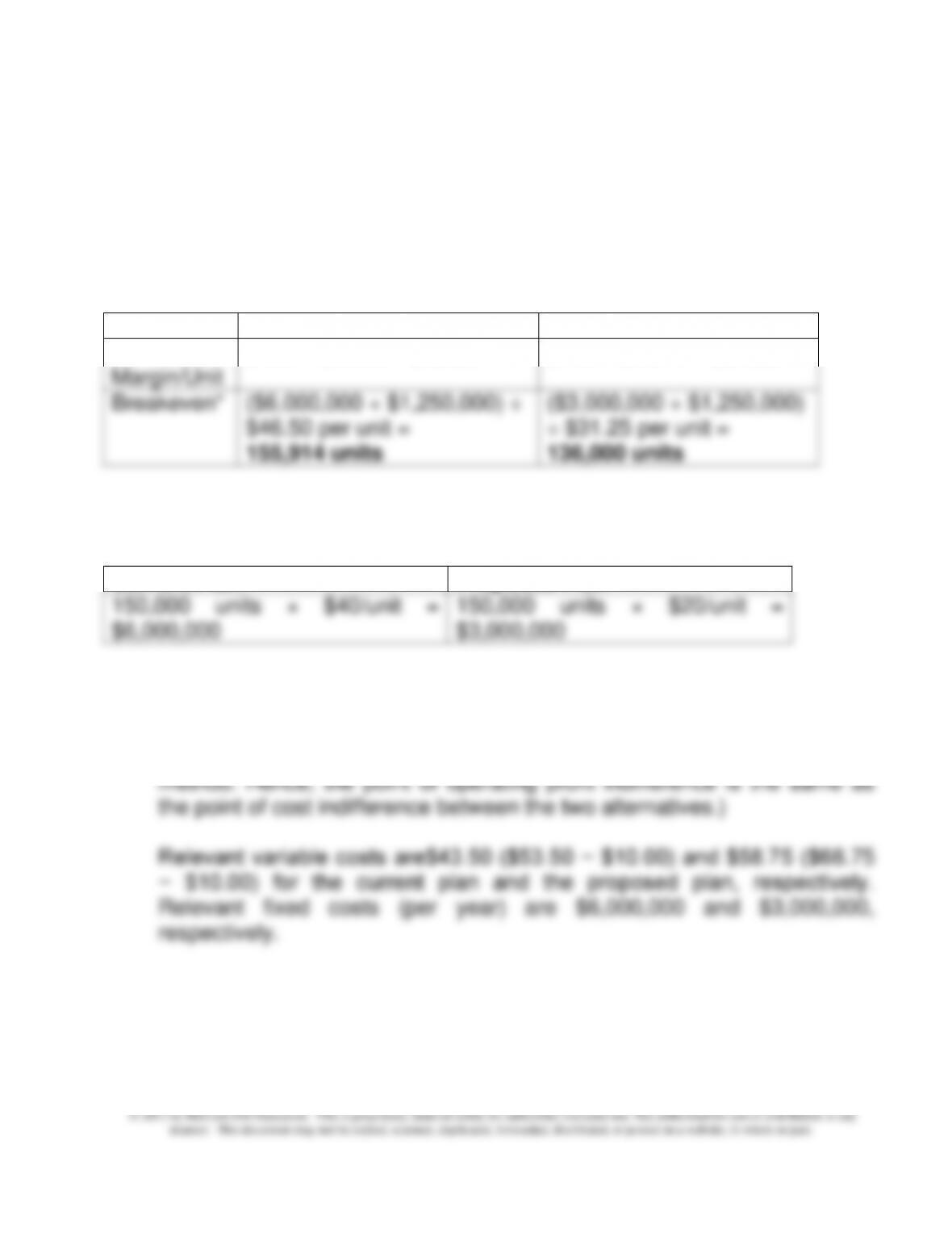
1. Total variable costs per unit for the current plan are
$6+$12.50+$25+$10=$53.50, and $15+$13.75+$30+$10=$68.75 under
the proposed plan. Thus, the contribution margin per unit and breakeven
point (in units) for each of the two plans are as follows:
Current Plan
Proposed Plan
Contribution
Margin/Unit
$100 − $53.50 = $46.50
$100 − $68.75 = $31.25
Breakeven*
($6,000,000 + $1,250,000) ÷
$46.50 per unit =
155,914 units
($3,000,000 + $1,250,000)
÷ $31.25 per unit =
136,000 units
*Fixed manufacturing overhead costs are determined from the fixed
overhead rates:
Current Plan
Proposed Plan
150,000 units × $40/unit =
$6,000,000
150,000 units × $20/unit =
$3,000,000
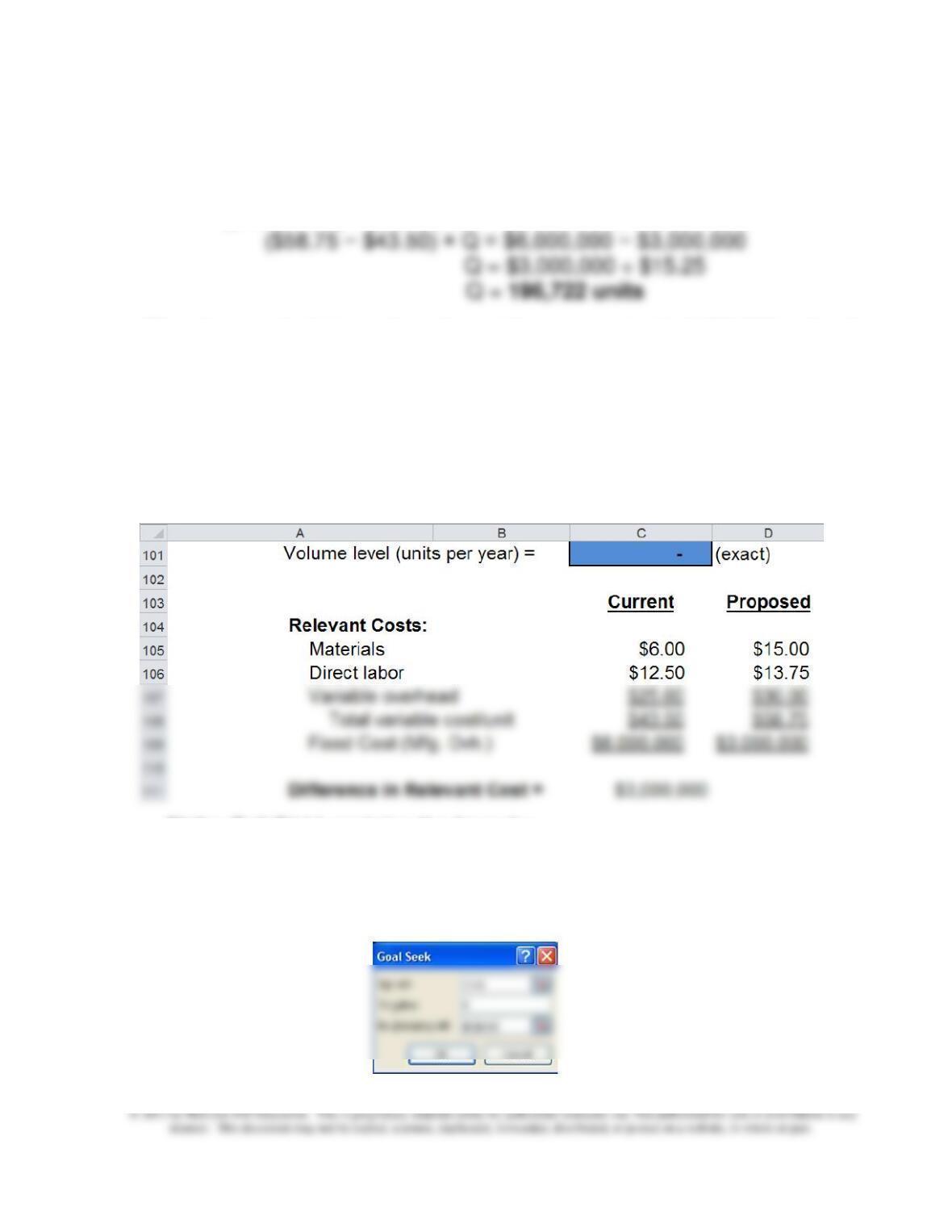
2. To determine the sales volume (in units) at which CG would be indifferent
between the current manufacturing plan and the proposed plan, solve for
the point, Q, in which total relevant cost is the same for the two decision
alternatives. (Revenue from sales is unaffected by choice of production
The indifference point, Q, can be found at the point of cost equality, as
follows:
Chapter 9 – Short-Term Profit Planning: Cost-Volume-Profit (CVP) Analysis
9-58
9-46 (Continued-1)
Total Relevant Cost, Current = Total Relevant Cost, Proposed
($43.50 × Q) + $6,000,000 = ($58.75 × Q) + $3,000,000
(The above calculations show that at the current level of 150,000 units, the
firm would prefer the low-fixed-cost strategy, that is, the new plan.)
3. Use Goal Seek in Excel to confirm the answer found above in Requirement
2:
Step #1: Define the Cost-Differential Equation (i.e., Relevant Cost of
Current Production Plan – Relevant Cost of Proposed Plan)
Note: Cell C111 contains the formula:
((C101*C108) + C109) – ((C101*D108) + D109)
Step #2: Run Goal Seek, as follows:
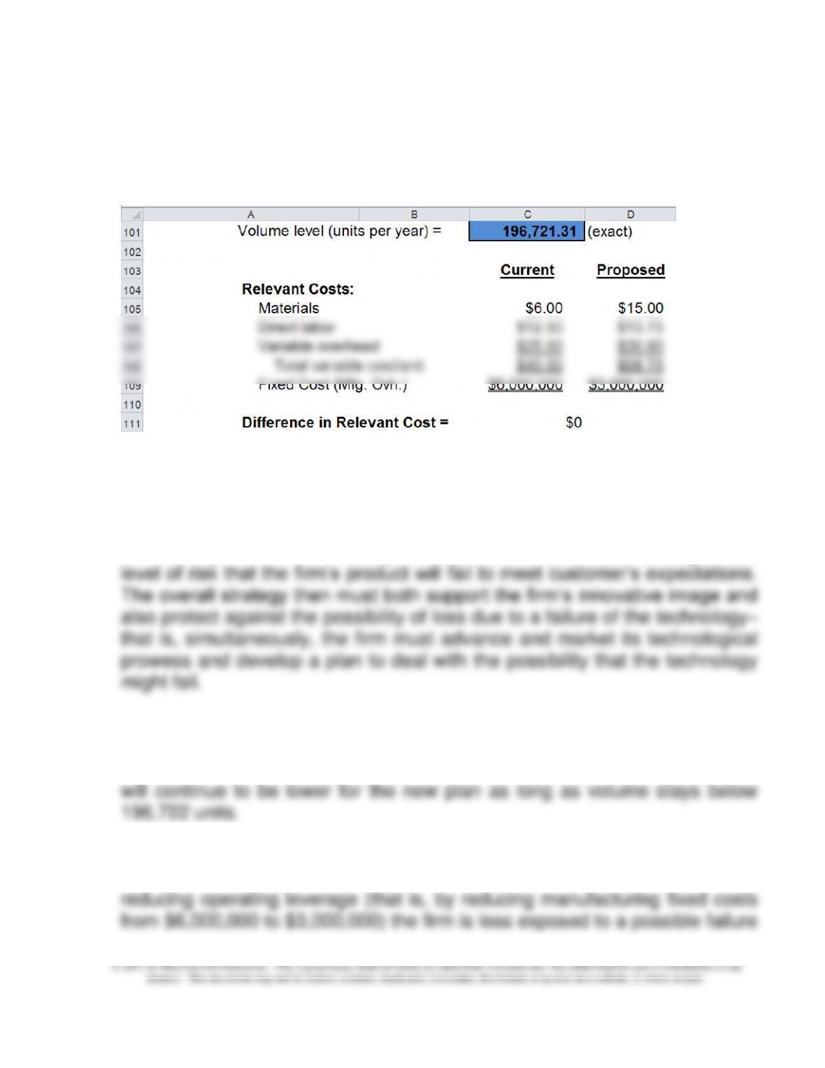
Chapter 9 – Short-Term Profit Planning: Cost-Volume-Profit (CVP) Analysis
9-59
9-46 (Continued-2)
Step #3: Generate Results, as follows:
4. CG’s strategy is best described as differentiation, since the firm has
succeeded by innovation in product design. Further, the firm operates in an
industry in which innovation and product design are critical to success. An
important element of the firm’s strategy is also the fact that the technology,
as for many firms in the industry, is not proven. That is, there is a significant
5.
a) The calculations in part 2 above support a decision to go to the new plan;
at the current level of 150,000 units, costs are lower for the new plan, and
b) Thinking strategically, the new plan is also preferred since it is an
appropriate response to the firm’s risk, as noted in Part 3 above. By
Chapter 9 – Short-Term Profit Planning: Cost-Volume-Profit (CVP) Analysis
of the innovation and the drop off in sales. The reduction in fixed costs also
helps the firm to manage cash flows. Thus, the new plan is more consistent
Also, one could look at the proposal as consistent with the firm’s core
strength, which appears to be product innovation. There is no evidence that
the firm is particularly innovative or cost-effective in manufacturing. Thus, a
strategy which goes to less focus on manufacturing would be consistent
with this strategy; more focus should be retained in product design and
development.
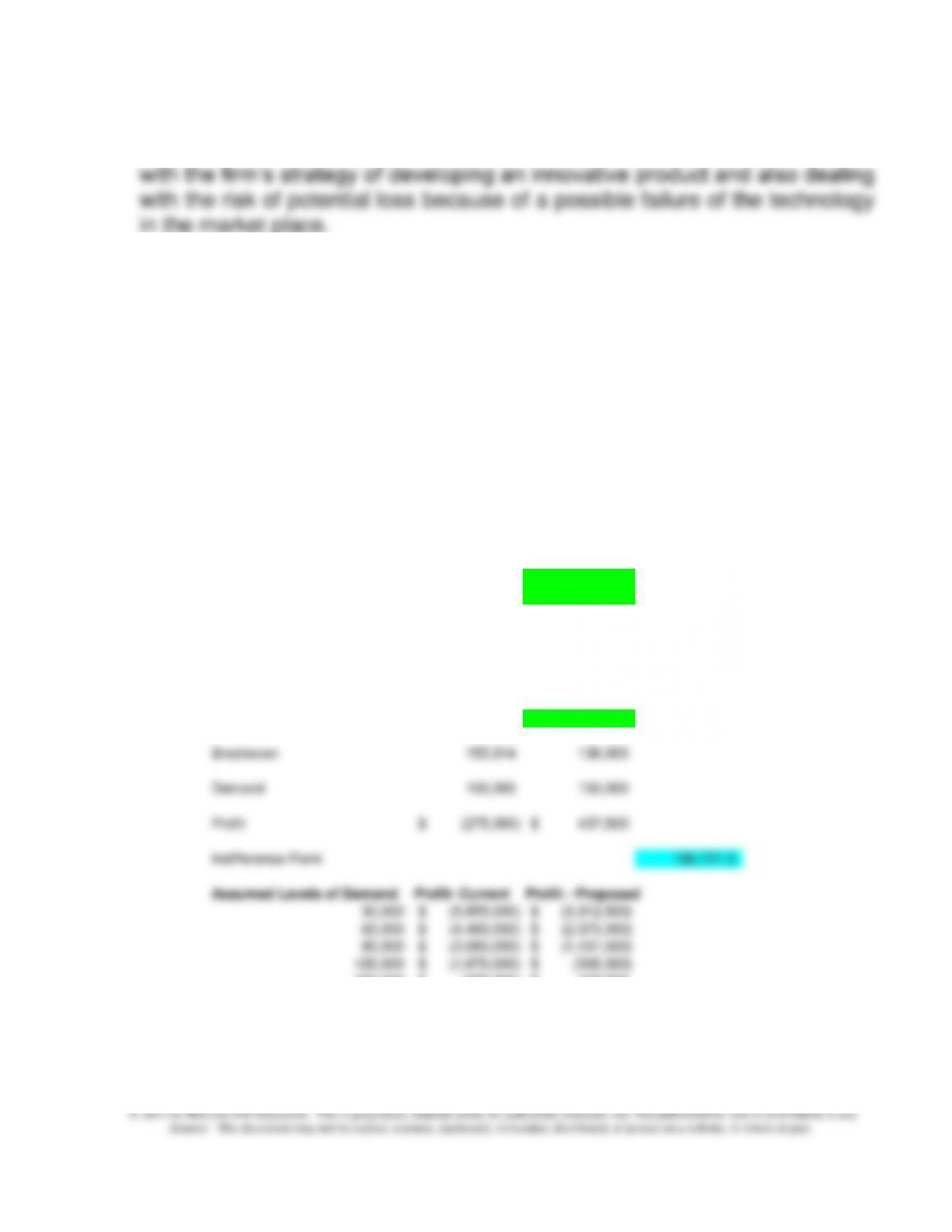
c) Sensitivity analysis: since uncertainty is important in this case, CG
Graphics should use some of the tools as illustrated below. Note that the
current method looks good if projected demand rises.
Current Proposed Difference
Materials and purchased parts 6.00$ 15.00$
Direct labor 12.50 13.75
Variable GS&A 10.00 10.00
Variable overhead 25.00 30.00
Total Variable cost 53.50$ 68.75$ 15.25$
Price 100 100
CM 46.50$ 31.25$
Fixed Cost 7,250,000.00$ 4,250,000.00$ 3,000,000$