Unlock document.
This document is partially blurred.
Unlock all pages and 1 million more documents.
Get Access
Chapter 9 - Short-Term Profit Planning: Cost-Volume-Profit (CVP) Analysis
9-12
Case 9-5: Sensitivity Analysis: Regression Analysis
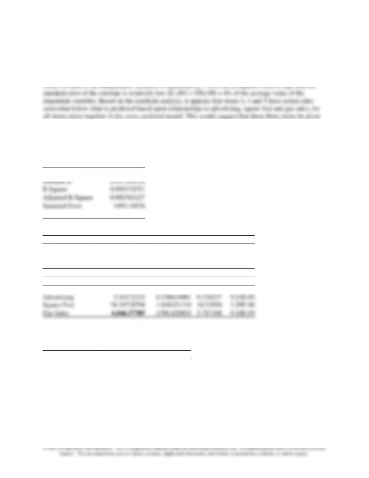
1. The regression analysis to identify the stores that seem to be operating at below their potential, based
on relationships for all the stores can be determined from a cross-sectional regression. The results are
shown below. Note that the regression has excellent measures for both reliability and precision. The t
some further study to determine whether (a) there is some variable omitted from the model which would
explain why these stores have relatively low sales, or (b) whether in fact the managers at these locations
have simply not been as effective as other managers in producing sales at their locations.
Note also that whether or not a store sell gasoline has a significant effect on total sales. For this data it
appears that gasoline contributes approximately $6,406 to total sales for locations selling gasoline.
Regression Statistics
Multiple R
0.997584458
R Square
0.995174751
Adjusted R Square
0.992762127
Standard Error
1993.16876
Observations
10
ANOVA
df
SS
MS
F
Regression
3
4916081167
1.64E+09
412.48641
Residual
6
23836330.24
3972722
Total
9
4939917497
Coefficients
Standard Error
t Stat
P-value
Intercept
-35228.92782
2772.415138
-12.70695
1.46E-05
Advertising
3.10172132
0.338644081
9.159237
9.54E-05
Square Feet
34.24728794
1.848351118
18.52856
1.59E-06
Gas Sales
6,046.57305
1596.620035
3.787108
9.10E-03
Having gas sales adds an estimated $6,046 in additional sales.
RESIDUAL OUTPUT
Observation
Predicted Sales
Residuals
1
57,299
(1,265)
2
22,181
864
3
88,073
1,264
4
68,005
(1,932)
5
21,970
(2,977)
6
64,160
766
7
27,792
981
8
44,713
1,581
9
74,410
(864)
9-13
10
35,386
1,582
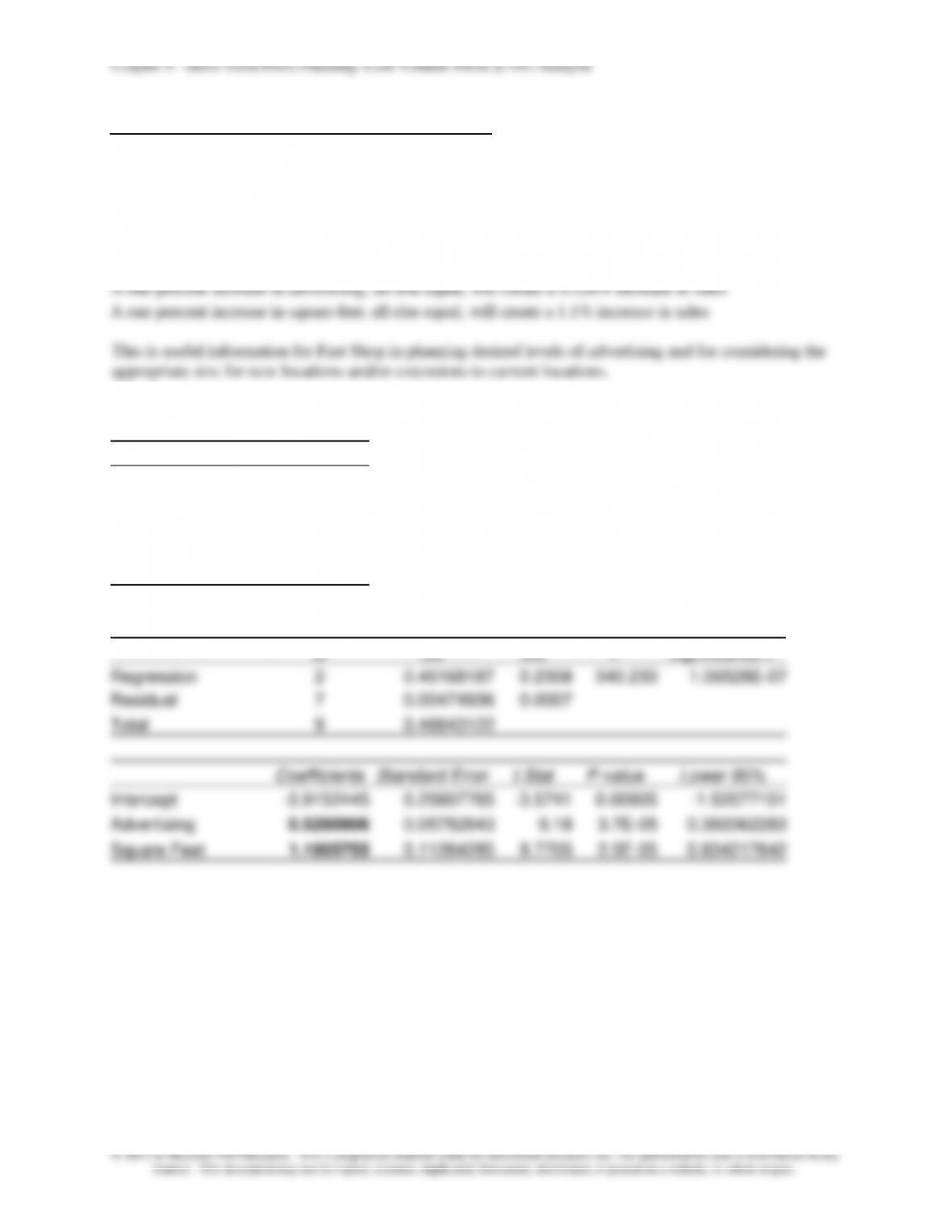
2. The analysis of the sensitivity of total sales to store size (square feet) and advertising can be
determined by taking the log transform for each of the data points and recalculating the regression. Note
again that the statistical measures for the regression are all excellent. Using the coefficients of the
independent variables, we can now find that:
A one percent increase in advertising, all else equal, will create a 0.528% increase in sales
A one percent increase in square feet, all else equal, will create a 1.1% increase in sales
This is useful information for Fast Shop in planning desired levels of advertising and for considering the
appropriate size for new locations and/or extensions to current locations.
Regression with Log Transforms on All Variables, except the Gas Sales (0,1) Variable
Regression Statistics
Multiple R
0.9948958
R Square
0.9898177
Adjusted R Square
0.9869084
Standard Error
0.0260476
Observations
10
ANOVA
df
SS
MS
F
Significance F
Regression
2
0.46168187
0.2308
340.233
1.06528E-07
Residual
7
0.00474936
0.0007
Total
9
0.46643122
Coefficients
Standard Error
t Stat
P-value
Lower 95%
Intercept
-0.9152445
0.25607765
-3.5741
0.00905
-1.52077151
Advertising
0.5280906
0.05752643
9.18
3.7E-05
0.392062283
Square Feet
1.1005755
0.11264285
9.7705
2.5E-05
0.834217642
Chapter 9 - Short-Term Profit Planning: Cost-Volume-Profit (CVP) Analysis
9-14
Case 9-6: Profit Planning—Choice of Cost Structure
Note to Instructor:
For those students seeking to become a Certified Management Accountant (CMA), the topic of CVP
analysis is an important one covered on the CMA exam. 1 In terms of this topic, the successful candidate
is expected to be able to:
▪ demonstrate an understanding of how cost/volume/profit (CVP) analysis is used to examine
the behavior of total revenues, total costs, and operating income as changes occur in output
levels, selling prices, variable costs per unit, or fixed costs
▪ differentiate between costs that are fixed and costs that are variable with respect to levels of
output
▪ demonstrate an understanding of the behavior of total revenues and total costs in relation to
output within a relevant range
▪ explain why the classification of fixed vs. variable costs is affected by the timeframe being
considered
▪ demonstrate an understanding of how contribution margin per unit is used in CVP analysis
▪ calculate contribution margin per unit and total contribution margin
▪ calculate the breakeven point in units and dollar sales to achieve targeted operating income or
targeted net income
▪ demonstrate an understanding of how changes in unit sales mix affect operating income in
multiple-product situations
▪ demonstrate an understanding of why there is no unique break-even point in multiple-product
situations
▪ analyze and recommend a course of action using CVP analysis
▪ demonstrate an understanding of the impact of income taxes on CVP analysis
Recommended Solutions
(1) What is meant by the term “short-term profit-planning” model, and how can such a model be
used by management? (That is, in what sense can this model be used to facilitate planning,
control, or decision-making by managers of an organization?)
Short term operating profit can be modeled as a function of five factors: (1) selling price per unit; (2)
variable cost per unit; (3) total (short-term) fixed costs; (4) sales volume; and, (5) sales mix. A short-
term profit planning model combines these factors into a predictive model, that is, a model that can be
▪ What volume of sales (in units or dollars) is needed to break even?
▪ What volume of sales (in units or dollars) is needed to achieve a particular level of profit,
either on a pre-tax or post-tax basis?
1 Certified Management Accountant Learning Outcome Statements (effective 7/1/04) (Updated 07-2008), available
at http://www.imanet.org.tw/img/CMALOS.pdf
Chapter 9 - Short-Term Profit Planning: Cost-Volume-Profit (CVP) Analysis
9-15
▪ What effect would a change in selling price per unit have on operating profit of all other
factors were held constant?
▪ It is worthwhile to reduce sales price per unit in exchange for an estimated increase in
volume?
▪ Which type of cost structure, one that has relatively high variable costs versus one that has
relatively high fixed costs, is preferable for an organization?
▪ What is the percentage change in the break-even point for a given percentage change in fixed
costs?
▪ At what volume level would the firm be indifferent between two alternative cost structures?
▪ What would be the impact on the break-even point if all factors remained the same except
variable costs per unit decreased by a given number of dollars or a given percent?
▪ From a risk perspective: how will projected operating profit be affected if volume is less than
predicted (e.g., 5% less, or 10% less)?
▪ What is the “margin of safety” (in dollars, units, or percentage) for the coming accounting
period?
▪ What is the likely effect on operating profits of a shift in sales (or service) mix?
Note that the organization’s CVP model can be depicted in equation form or in graphical form, of
which there are two alternative formulations: a cost-volume-profit graph, and a profit-volume graph.
(2) What is the definition of “fixed cost,” “variable cost,” “contribution margin ratio,”
“contribution margin per unit,” and “relevant range”?
The terms “fixed cost” and “variable cost” represent descriptions of cost behavior, that is, to
descriptions of how a given cost changes or reacts to changes in one or more cost drivers (activity
variables). A fixed cost, within an assumed range of activity or output, does not change in total as
activity changes. As such, we can say that a fixed cost is independent of changes in activity or output.
By contrast, a variable cost is one that changes in total as output or activity changes. On a per-unit-of-
some range of output/activity (the relevant range).
Contribution margin per unit represents the spread between the selling price per unit and the variable
cost per unit. It is the amount that the sale of each unit contributes toward the recovery of fixed costs,
and then profits. Contribution margin ratio is a percentage represented as the ration of contribution
margin per unit to selling price per unit. As such, it represents the proportion of each sales dollar that
is available for recovery of fixed costs, and then profit.
(3) What is the break-even point, in terms of number of deliveries per year (or per month), for
Alternative #1? For Alternative #2?
The break-even volume (X) (in this case # of deliveries) is given as:
X = Fixed Costs (FC) ÷ Contribution Margin per Unit (cm)
The break-even volume, per year, for Alternative #1 is:
Chapter 9 - Short-Term Profit Planning: Cost-Volume-Profit (CVP) Analysis
9-16
X = $600,000 ÷ $12 per unit = 50,000 units
(4) How many deliveries would have to be made under Alternative #1 to generate a pre-tax profit,
πB, of $25,000 per year?
The required sales volume (X) (in this case # of deliveries) is given as:
X = [Fixed Costs (FC) + πB] ÷ Contribution Margin per Unit (cm)
The required sales volume, per year, for Alternative #1 is:
(5) How many deliveries (per year) would have to be made under Alternative #1 to generate a pre-
tax profit, πB, equal to 15% of sales revenue?
We begin with the following general profit equation, where X = sales volume:
πB = TR – VC – FC
At annual volume of 200,000 units, TR = $12,000,000, VC = $9,600,000, and with FC = $600,000
the pre-tax operating income = $1,800,000, which is exactly 15% of total sales revenue, TR.
(6) How many deliveries would have to be made under Alternative #2 to generate an after-tax
profit, πA, of $100,0000 per year, assuming a tax rate of, say, 45%?
The required sales volume (X) (in this case # of deliveries) is given as:
X = [Fixed Costs (FC) + πB] ÷ Contribution Margin per Unit (cm)
where πB = πA ÷ (1 – t), where t = effective income-tax rate
πB = $100,000 ÷ (1 – 0.45) = $181,818
Chapter 9 - Short-Term Profit Planning: Cost-Volume-Profit (CVP) Analysis
9-17
(7) Assume that for the coming year total fixed costs are expected to increase by 10% for each of
the two alternatives. What is the new break-even point, in terms of number of deliveries, for
each decision alternative? By what percentage did the break-even point change for each case?
How do these figures compare to the percentage increase in budgeted fixed costs?
Alternative #1:
New Fixed Costs (per year) = $600,000 × 1.10 = $660,000
New Break-Even Point (in number of deliveries per year):
X = $660,000 ÷ $12 per unit = 55,000 units
Alternative #2:
New Fixed Cost (per year) = $3,000,000 × 1.10 = $3,300,000
New Break-Even Point (in number of deliveries per year):
The above calculations illustrate the following general rule: a given percentage change in fixed costs
translates to an equivalent percentage change in the break-even point.
(8) Assume an average income-tax rate of 40%. What volume (number of deliveries) would be
needed to generate an after-tax profit, πA, of 5% of sales for each alternative?
This question is an extension of question 5 (above) to the after-tax case. First, we note (as in 6 above)
that:
πB = πA ÷ (1 – t), where t = effective income-tax rate
For Alternative #1:
πB = 0.05($60X) ÷ (1 – 0.40) = $5X
As before, πB = TR – VC – FC
Chapter 9 - Short-Term Profit Planning: Cost-Volume-Profit (CVP) Analysis
9-18
X = 85,715 units
For Alternative #2:
πB = 0.05($60X) ÷ (1 – 0.40) = $5X
$25X = $3,000,000
X = 120,000 units
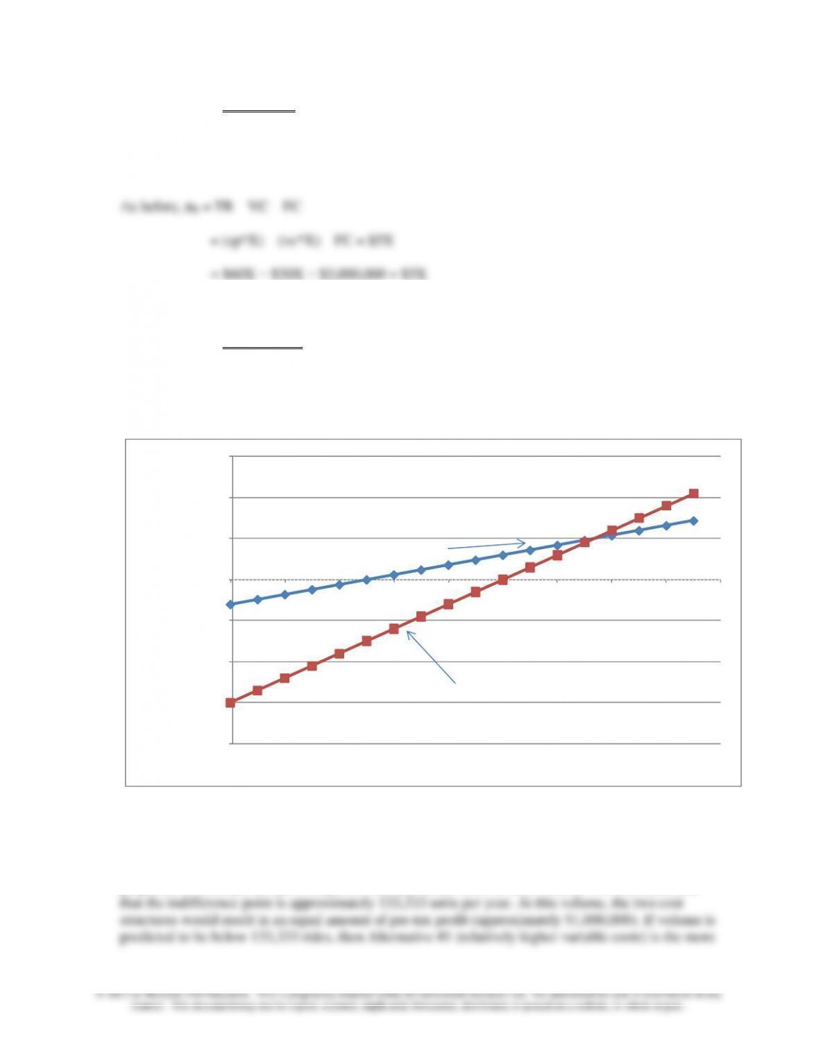
(9) Consider the original data in the problem. Construct a graph for each of the two alternatives
depicting pre-tax profit, πB, as function of volume (number of deliveries per year). Clearly label
the profit equation for each alternative.
$(4,000)
$(3,000)
$(2,000)
$(1,000)
$-
$1,000
$2,000
$3,000
-20 40 60 80 100 120 140 160 180
Pre-Tax pofit (Thousands)
Number of Delveries (D) per year (000s)
-$600,000 + $12D
-$3,000,000 + $30D
(10) Based on the graphs prepared in (9), which decision-alternative do you think is the more
profitable one for this business?
We cannot say which firm’s cost structure is more profitable because, as indicated by a general CVP
graph, the level of pre-tax profit depends crucially on the level of sales volume. We can determine
Chapter 9 - Short-Term Profit Planning: Cost-Volume-Profit (CVP) Analysis
9-19
profitable of the two. However, if sales are expected to exceed 133,333 units per year, then
Alternative #2 leads to more profits.
(11) Based on the original data and the graphs prepared above in (10), which decision alternative is
more risky to the business? Explain. (Hint: Think about, and define in your answer, the notion
of “operating leverage.”)
The contribution margin generated from sales must be sufficient to cover the fixed costs; any excess
after coverage of fixed costs translates directly into pre-tax profit. If the contribution margin is not
sufficient to cover the fixed costs, then a loss occurs for the period. That is, cost structures with
relatively higher amounts of fixed costs are riskier, just as firms with relatively high levels of debt in
to increase sales volume. This is particularly true of the company is currently operating near the
break-even point. In this case, even small percentage changes in sales volumes lead to dramatic
percentage changes in pre-tax profit—in both directions.
Note, however, that once the breakeven point has been reached, pre-tax profit increases by the
product of the unit contribution margin and the number of units sold. Thus, as seen from the above
graph, if volume is predicted to be high, the preferred cost structure is Alternative #2. Once the break-
even point is reached, a large portion of each sales dollar goes directly to operating income.
(12) Finally, in building your profit-planning (i.e., CVP) model, the analyst makes a number of
important assumptions. List the primary assumptions that underlie a conventional CVP
analysis, such as the ones you conducted above.
Any model is only as good (accurate) as the validity of the underlying assumptions of the model. The
following are the assumptions behind a traditional CVP model:
1. Revenues and costs (variable and total) change only in response to a single driver:
volume of sales. In fact, the term CVP derives precisely from this assumption.
Chapter 9 - Short-Term Profit Planning: Cost-Volume-Profit (CVP) Analysis
9-20
Case 9-7: Pancake World
Note to Instructor: The Pancake World Case is based on the actual experience and disguised data of a
franchise owner of one of the well-known pancake restaurants.
1) From the information that the annual number of guests, it is possible to get the average variable
cost per guest of $3.82 = $497,000 ÷ 130,000. Since the average ticket price per guest is $7.45,
breakeven in number of guests can be calculated as follows.
Fixed Costs ÷ (Selling Price − Variable cost) = number to break even
Weekend average guest count is 633 guests. The difference is 422 guests from the breakeven
guest count. Louis sees a good safety margin.
Weekends tend to be busier than weekdays. Also, when holidays fall on a weekday this brings up
guest count and expenses. The annual breakeven gives a useful figure for planning. While
demand varies during the week, variable costs (food and labor) follow the demand, and fixed
costs tend to be monthly and/or annual. So, seasonality plays a minor role in breakeven analysis
over the course of a year.
2) Referring to Exhibit 3 under the Labor % row gives labor % breakdown per day. Calculating the
average for the week a figure of 22.5% labor cost has been achieved. This is one percentage point
other hand, a key feature of the cost structure of the restaurant is that most costs are variable,
food and labor, so that it is difficult to achieve a high degree of operating leverage. One thing
that helps is to outsource some types of labor (e.g., payroll processing) and outsource some
aspects of food inventory (food delivery, by U.S. Foodservice Inc.) to allow the restaurant to
focus on customer service and improving customer loyalty.

Chapter 9 - Short-Term Profit Planning: Cost-Volume-Profit (CVP) Analysis
9-21
Teaching Strategy for Readings
Reading 09-01: “Tools for Dealing with Uncertainty”
This article explains how to use simulation methods within a spreadsheet program such as Excel to
perform sensitivity analysis for a given decision context. The available spreadsheet simulation software
systems include the programs Crystal Ball and @Risk, among others. These software systems allow the
user to analyze the effect of uncertainty on the potential outcomes of a decision. These tools can be
applied directly to CVP analysis. The tools allow the user to see the potential effect on the breakeven
level or total profit of potential variations in the key uncertain factors in the analysis. The uncertain
factors affecting breakeven might be the unknown level of unit variable cost, price or fixed cost. Also, in
determining total profit, the unknown level of demand might be a key uncertain factor.
Exercise: Use a spreadsheet simulation tool such as Crystal Ball or @Risk to analyze the uncertain
factors in given case situation. Cases 9-1, 2 and 3 could be used or a problem from the text, for example,
Text problem 9-53, the Computer Graphics Case. This is illustrated in the “Advanced Lecture Notes”
section of the Instructor’s Resource Guide for Chapter 9.
Chapter 9 - Short-Term Profit Planning: Cost-Volume-Profit (CVP) Analysis
9-22
Reading 09-2: Turning Budgets into Business—Part I of III
Introductory Note: This assignment assumes familiarity with the comprehensive master budget exercise
developed by Porter and Stephanson (see Strategic Finance, February–July, 2010). The Excel solution
file containing this master budget, and obtained from by the authors from Porter and Stephanson, is
inserted as an object below:
Bob's Bicycles -
Master Budget.xlsx
In addition, the following pdf file (which contains data and assumptions needed to construct the master
budget for Bob’s Bicycle) can be distributed to students in advance of covering the requirements of
Reading 09-02:
The purpose of Reading 09-02 is to have students use the Master Budget (which was highlighted in the
set of Budgets by Porter &Stephanson that were published in Strategic Finance during 2010—see
solution file above) do the following:
1. Add a Contribution Margin Income Statement to the aforementioned Master Budget.
2. Using the fixed-and variable cost information provided by this Income Statement, we’ll calculate the
breakeven point and margin of safety and discuss how these two important numbers can be used in
decision making.
Student Lecture
Handout (Master Bud


