8-56
8-54 (continued –1)
2. The limitations of this regression are somewhat unique since the
independent variables (except for average pay) and the dependent
variable are rankings (ordinal numbers rather than real numbers).
Thus, the issue of nonlinearity arises, but in a different manner than
in most regressions applications. As noted in the text, nonlinearity
often arises because of trend or seasonality in the data when the data
is from a time-series. In this case, the data is cross-sectional, so we
do not have time-series nonlinearity problems. However, the
not capture that difference. Our linear analysis assumes that the
rankings have equal increments, an assumption that is likely to be
wrong at least to some degree.
Chapter 8 – Cost Estimation
8-57
8-55 Cost Estimation; Regression Analysis (50 min)
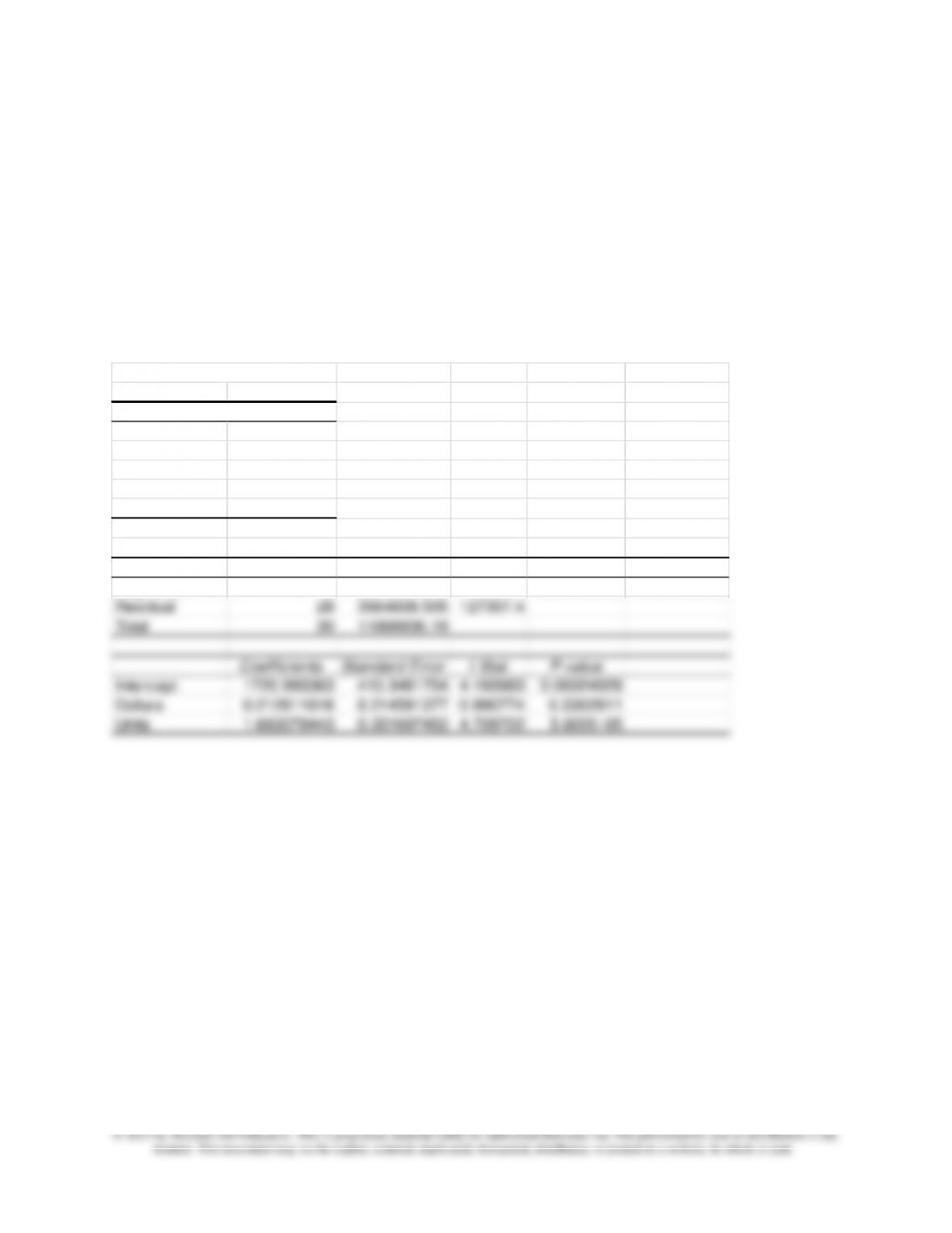
1. The spreadsheet regression output for Plantcity is shown in
Exhibits 8-55A, B and C. Exhibit 8-55A shows the regression which
includes both predictors, sales dollars and sales units, while Exhibit
8-55B shows sales dollars only, and Exhibit 8-55C shows sales units
only.
Exhibit 8-55A (Units and Dollars)
SUMMARY OUTPUT
Regression Statistics
Multiple R 0.836460729
R Square 0.699666551
Adjusted R Squa
0.678214162
Standard Error 356.8016909
Observations 31
ANOVA
df SS MS F
Significance F
Regression 2 8304227.689 4152114 32.6148545 4.85794E-08
Residual 28 3564608.505 127307.4
Total 30 11868836.19
Coefficients Standard Error t Stat P-value
Intercept 1720.993363 410.3481754 4.193983 0.00024928
Dollars 0.212611616 0.214591377 0.990774 0.3302811
Units 1.663079443 0.351697453 4.728722 5.822E-05
8-58
Problem 8-55 (continued –1)
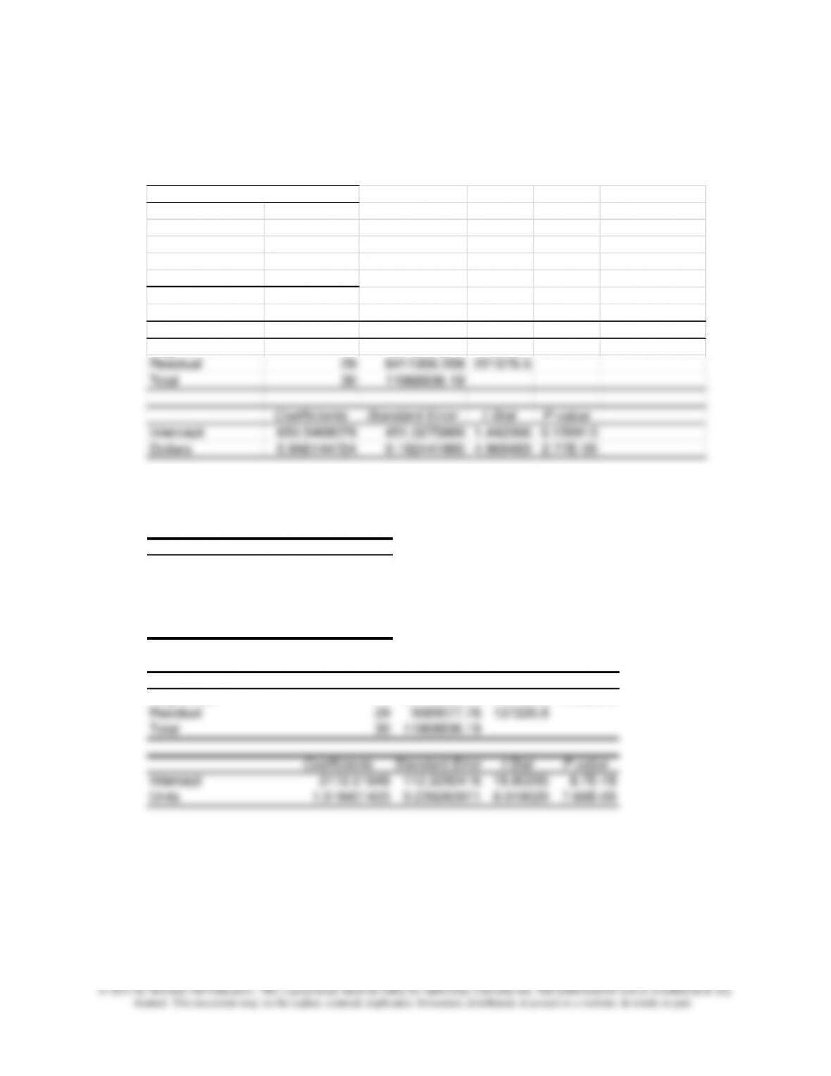
Exhibit 8-55B (Dollars)
Regression Statistics
Multiple R 0.678100395
R Square 0.459820145
Adjusted R Square 0.441193254
Standard Error 470.1909447
Observations 31
ANOVA
df SS MS F Significance F
Regression 1 5457529.985 5457530 24.68582 2.76888E-05
Residual 29 6411306.209 221079.5
Total 30 11868836.19
Coefficients Standard Error t Stat P-value
Intercept 650.5468079 451.0275889 1.442366 0.159913
Dollars 0.956144724 0.192441985 4.968483 2.77E-05
Exhibit 8-55C (Units)
Regression Statistics
Multiple R 0.830142974
R Square 0.689137358
Adjusted R Square 0.678417956
Standard Error 356.6886878
Observations 31
ANOVA
df SS MS F
Regression 1 8179258.414 8179258 64.28879
Residual 29 3689577.78 127226.8
Total 30 11868836.19
Coefficients
Standard Error
t Stat P-value
Intercept 2112.01648 112.3290416 18.80205 8.7E-18
Units 1.918401433 0.239260971 8.018029 7.66E-09
Chapter 8 – Cost Estimation
8-59
8-55 (continued –2)
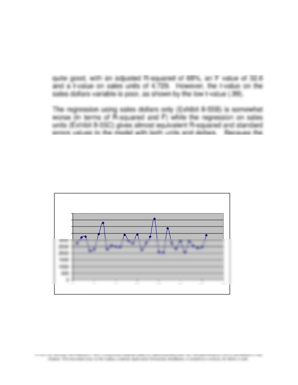
The precision of the regression shown in 8-55A is good, with a
standard error of the estimate of 357 relative to a dependent variable
with values averaging about 3,000. Also, the reliability of the model is
errors values to the model with both units and dollars. Because the
regression on sales units only is simpler and has a lower standard
error and higher R-squared, the model using only sales units is a
logical choice for the cost estimation model in this case.
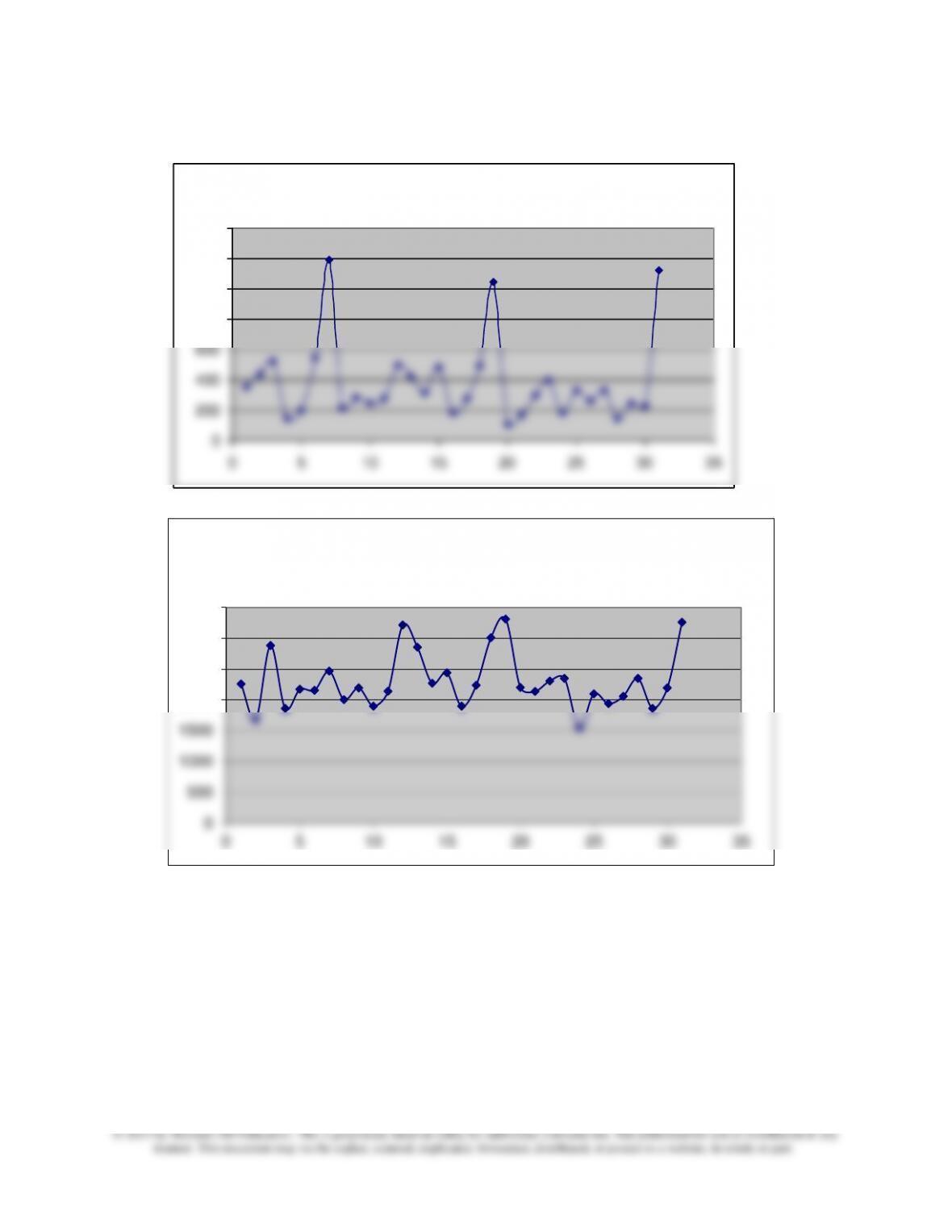
For further regression analysis on this data, consider the graphs
below which shows evidence of seasonality in the data.
Expense
0
500
1000
1500
2000
2500
3000
3500
4000
4500
5000
0 5 10 15 20 25 30 35
8-60
8-55 (continued –3)
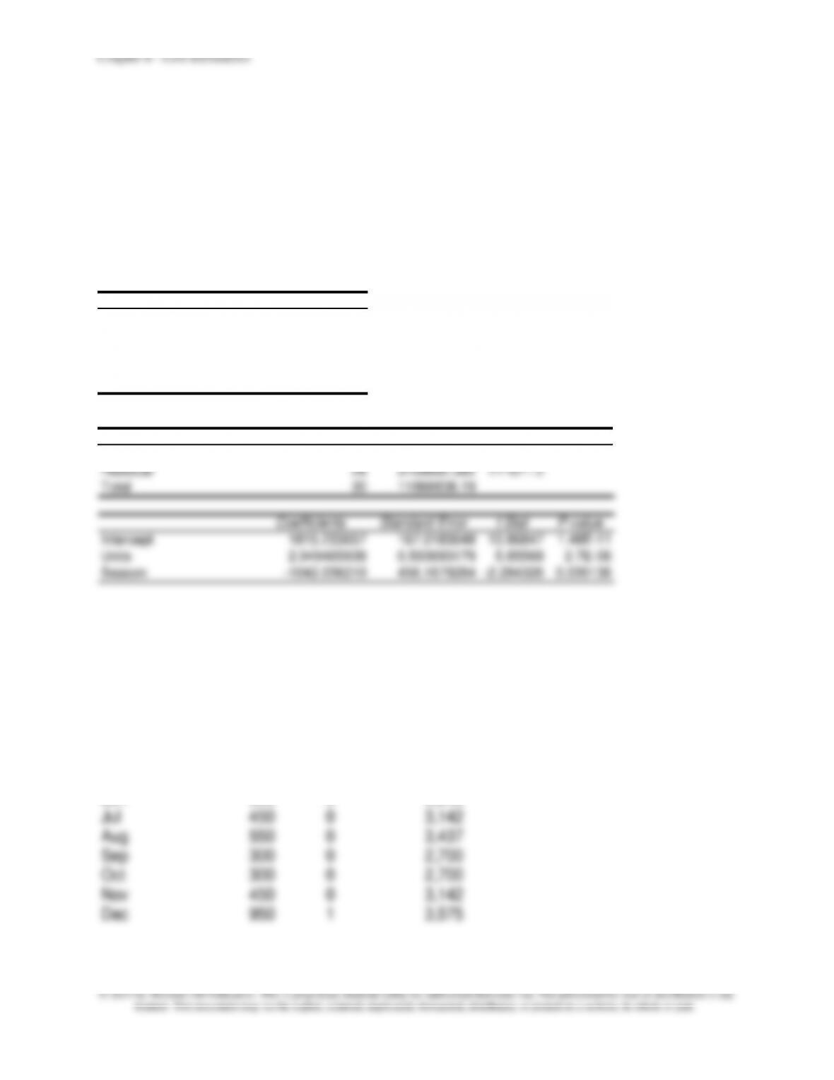
Since the graphs show clear evidence of seasonality, another try of
the model with seasonality included would be a useful next step. The
addition of a seasonal variable for the month of December improved
the model in Exhibit 8-55C substantially.
Units
0
200
400
600
800
1000
1200
1400
0 5 10 15 20 25 30 35
0
500
1000
1500
2000
2500
3000
3500
0 5 10 15 20 25 30 35
Dollars
8-61
8-55 (continued -4)
The seasonal model is shown in Exhibit 8-55D. Note the substantial
improvement in R-squared; also note that the seasonal variable is
significant. The coefficient on the seasonality variable is negative
because supplies expense does not rise as fast as units sold in
December.
Exhibit 8-55D
Regression Statistics
Multiple R 0.859051742
R Square 0.737969895
Adjusted R Square 0.719253459
Standard Error 333.2733966
Observations 31
ANOVA
df SS MS F
Regression 2 8758843.802 4379422 39.42898
Residual 28 3109992.392 111071.2
Total 30 11868836.19
Coefficients Standard Error t Stat P-value
Intercept 1815.233657 167.0183648 10.86847 1.48E-11
Units 2.949465938 0.503693179 5.85568 2.7E-06
Season -1042.036219 456.1679284 -2.284326 0.030136
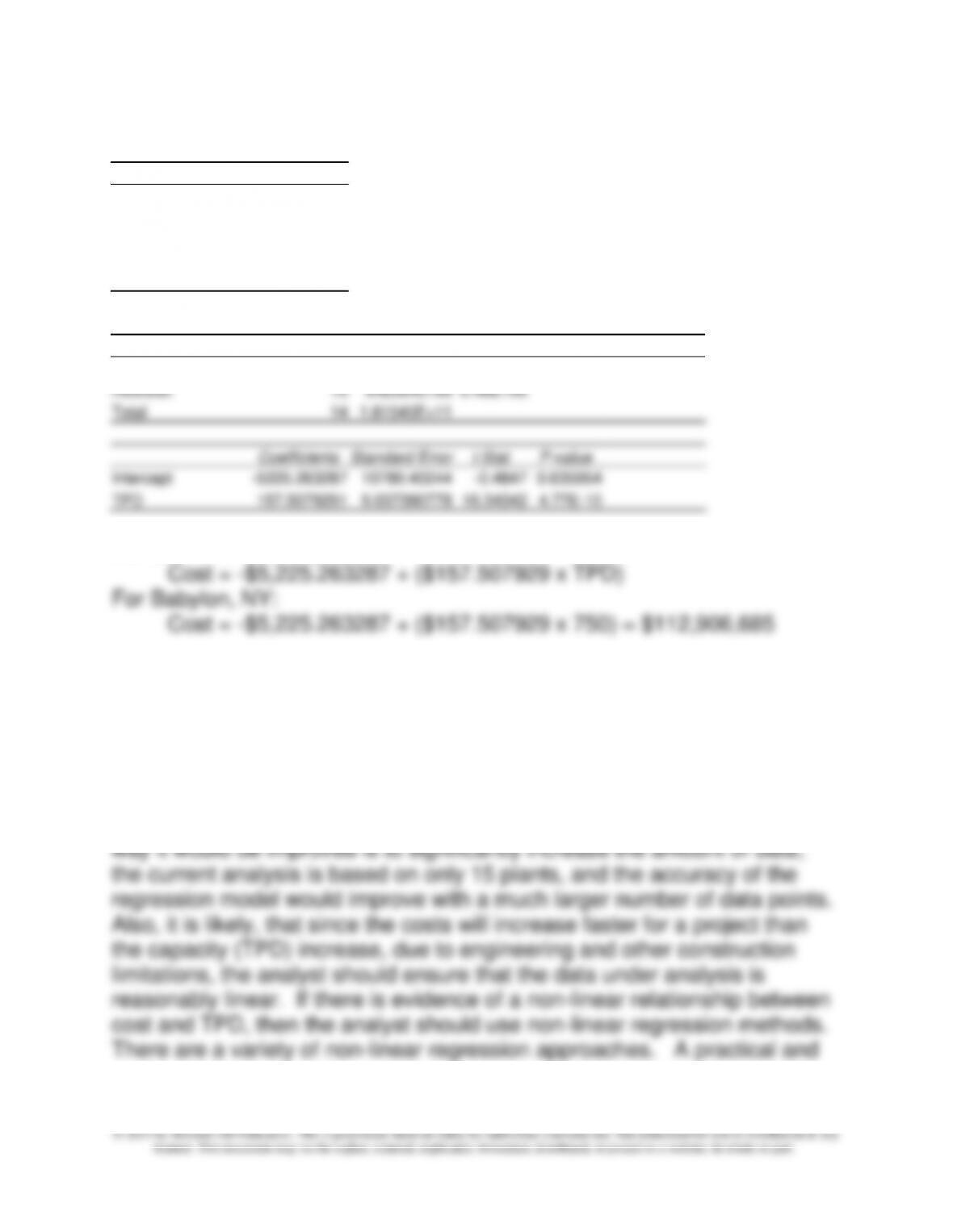
2. Predicted monthly figures for supplies expense using the
regression in Exhibit 8-55D:
Units Seasonality Predicted Expense
Jan 180 0 2,346$
Feb 230 0 2,494
Mar 190 0 2,376
Apr 450 0 3,142
May 350 0 2,848
Jun 350 0 2,848
Jul 450 0 3,142
Aug 550 0 3,437
Sep 300 0 2,700
Oct 300 0 2,700
Nov 450 0 3,142
Dec 950 1 3,575
8-62
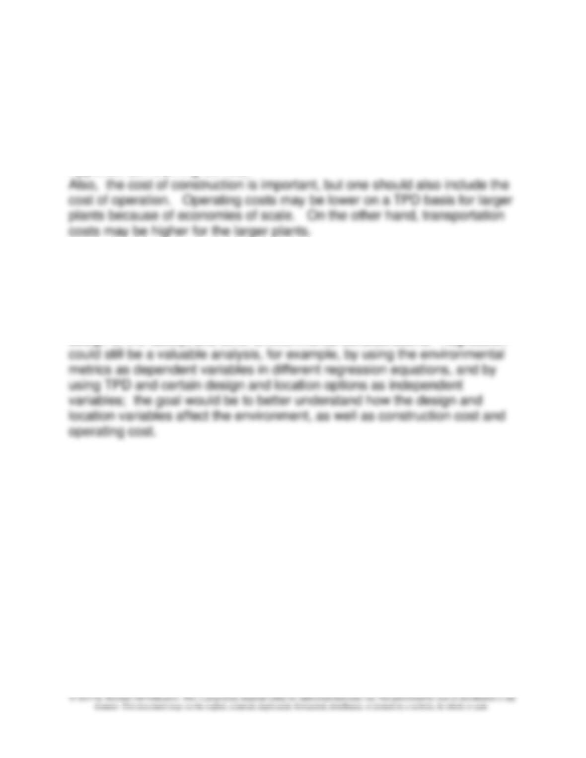
8-56 Cross-Sectional Regression (30 min)
1.
Regression Statistics
Multiple R
0.976518934
R Square
0.953589229
999
Adjusted R Square
0.95001917
Standard Error
25458.32309
Observations
15
ANOVA
df
SS
MS
F
Significance F
Regression
1
1.73119E+11
1.73E+11
267.1074
4.77053E-10
Residual
13
8425640789
6.48E+08
Total
14
1.81545E+11
Coefficients
Standard Error
t Stat
P-value
Intercept
-5225.263287
10780.40244
-0.4847
0.635954
TPD
157.5079291
9.637390778
16.34342
4.77E-10
Construction Cost Equation
2. The regression has strong statistical measures. The R-squared is
relatively high at 95.35%; the t-value for the independent variable TPD is
high and the risk level (p) is low; the standard error of the estimate, at
25,458, is relatively small given the amounts predicted for the dependent
variable, so overall, the regression looks very strong, and the management
accountant should feel comfortable to rely on it in cost estimation. One
Chapter 8 – Cost Estimation
8-63
simple to apply method is to convert the data by taking the natural log (ln)
of each data point and then running the regression with the logged data.
8-56 (continued -1)
The conversion of logs removes the multiplicative type of non-linearity from
the equation. To see this, review the discussion in footnote 14 in the
Appendix (on learning curves).
3. From the standpoint of sustainability, the focus of the analysis needs to
move from construction costs to environmental metrics that measure the
effect on ground water, air quality, overall energy consumption in the
process of wastewater treatment, and other environmental variables. This
would add to the analysis such factors as the location of the facility, the
design of the facility, and other environmental considerations. Regression
Source: Richard K. Ellsworth, “Cost–to-Capacity Analysis for Estimating
Project Costs,” Construction Accounting and Taxation, September/October
2005, pp 5-10.
8-64
8-57 Cost Estimating for Defense Contracting; Using the Internet (25
min)
1.The cost estimation methods described in the document are called CERs
(cost estimating relationships) which are defined as mathematical
expressions relating the cost as the dependent variable to one or more
independent variables. The CERs described in the document include
simple and multiple linear regression and curvilinear regression. Cost
aviation industry.
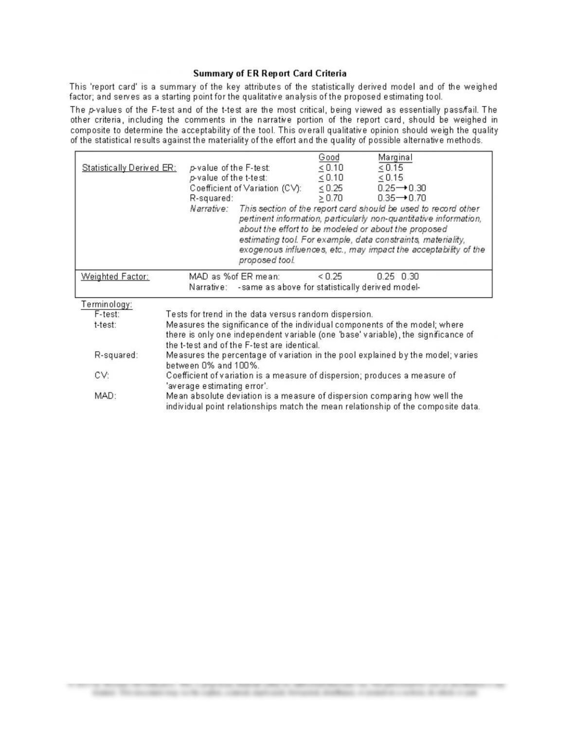
2. The model validation criteria in “Summary of ER Report Card Criteria” on
p 84 in chapter 3 of the handbook are very similar to those suggested in the
text for most statistical measures, and less restrictive than the text for other
measures. For example, the requirements for R-square are relatively
The “Summary of ER Report Card Criteria” is shown on the following page.
Chapter 8 – Cost Estimation
8-65