Chapter 8 – Cost Estimation
8-31
8-42 (continued – 3)
3.
The Gilmore company is likely to have a number of sustainability
issues in its business. As a company that renovates older homes, it
must frequently deal with hazardous materials such as asbestos used
in siding and other construction materials decades ago. Current
construction codes require renovations of older homes to treat the
hazardous materials with special, sometimes expensive procedures.
The removal and proper disposal of the materials must be carefully
and effectively done in compliance with local, state, and federal
The role of cost estimation is important when a construction company
such as the Gilmore company must accurately budget costs for
renovations in making bids and in dealing with the occasional
unexpected problems. Careful cost estimates can help Gilmore to
more effectively prepare bids and proposals for new work, and to
increase profitability along the way.
8-32
8-43 Cost Estimation; Machine Replacement; Ethics (25 min)
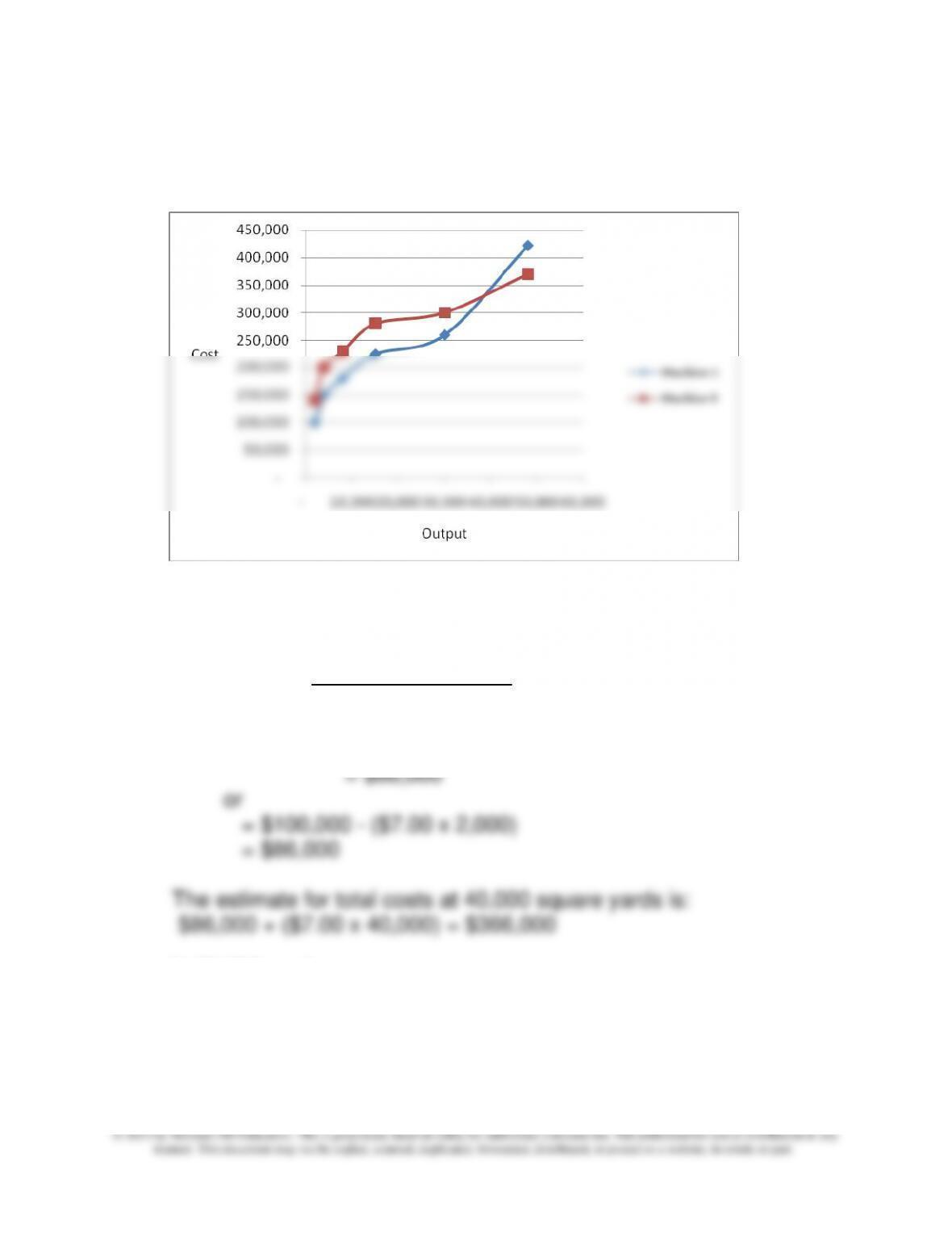
1. A graph of the data shows no significant outliers nor nonlinear
relationships. See below
Using the High-Low method:
Machine A:
slope = $422,000 – $100,000 = $7.00
48,000 – 2,000
constant = $422,000 – ($7.00 x 48,000)
At 25,000 yards:
$86,000 + ($7.00 x 25,000) = $261,000
8-33
8-43 (continued -1)
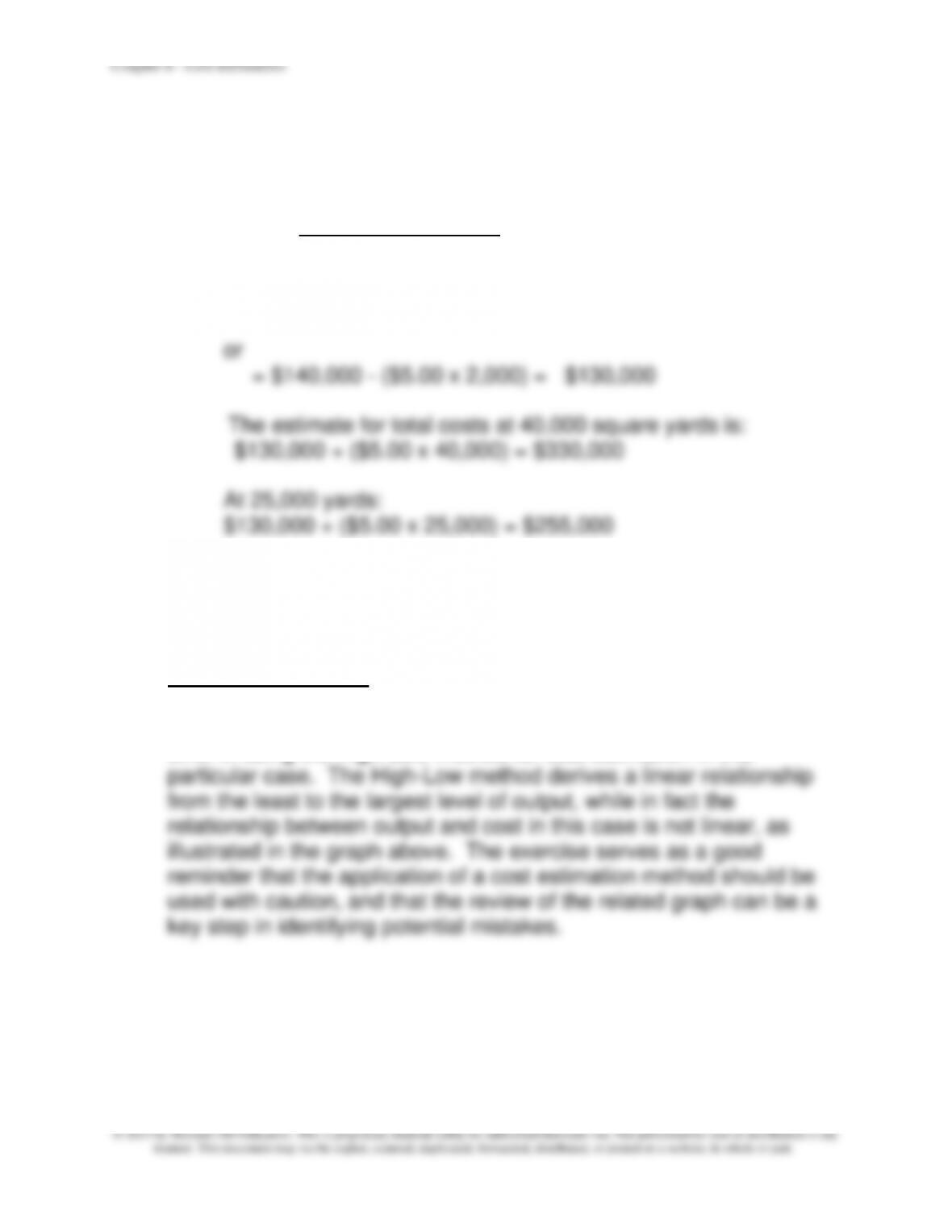
Machine B:
slope = $370,000 – $140,000 = $5.00
48,000 – 2,000
constant = $370,000 – ($5.00 x 48,000) = $130,000
The calculations show that the costs are lower at both the 40,000
and the 25,000 level for Machine B, which suggest that Machine B is
preferred to Machine A for production levels above at least 25,000.
The answer is wrong. Note by inspection of the chart in the text and
inspection of the graph above, that Machine A is preferred to Machine
B up to approximately 40,000 units. The error in the analysis is the
error in using the High-Low method for cost estimation in this
8-34
8-43 (continued -2)
2. The ethical issue presented in this case should be addressed using
the approach described in chapter 1. Here it seems important to
consider the nature and extent of the effect of the defect on
customers and also GlasTech. Since the glass is used in office
the calculations should not be modified.
3. In addition to the costs of the machine, GlasTech should be aware
of any import duties or restrictions for the purchase of the machines
from Germany or Canada. How will these restrictions and duties, if
country might open up new markets for GlasTech.
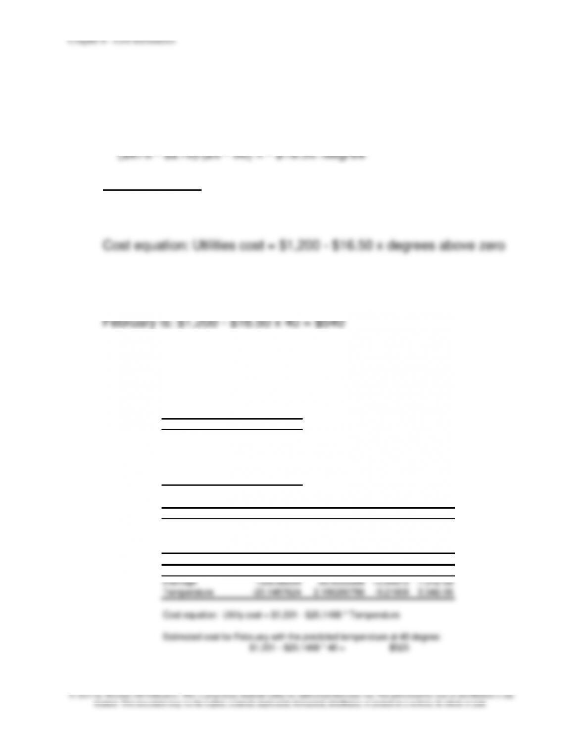
8-44 Cost Estimation; High-Low Method (25 min)
Estimated cost of electricity equals $210 (from information about
August)
At 20 degrees F:
$870 = intercept + (-$16.50 x 20)
intercept = $1,200
A cost estimate for January is not available since the average
temperature of 10 degrees is outside the relevant range of the data
used to develop the high-low estimate. The cost estimate for
February is: $1,200 – $16.50 x 40 = $540
Note to instructor: the problem can also be solved using regression
analysis, as shown below. Note that the predicted cost, $525, differs
from the High-Low method, but not significantly.
Regression Statistics
Multiple R 0.94586791
R Square 0.8946661
Adjusted R Square 0.88413271
Standard Error 80.2291185
Observations 12
ANOVA
df SS MS F
Regression 1 546709.8021 546709.8 84.9362
Residual 10 64367.1146 6436.711
Total 11 611076.9167
Coefficients Standard Error t Stat P-value
Intercept 1330.88094 95.4055084 13.94973 7.01E-08
Temperature -20.1487624 2.186260788 -9.21608 3.34E-06
Cost equation: Utility cost = $1,331 – $20.1488 * Temperature
Estimated cost for February with the predicted temperature at 40 degree:
$1,331 – $20.1488 * 40 = $525
8-36
8-44 (continued –1)
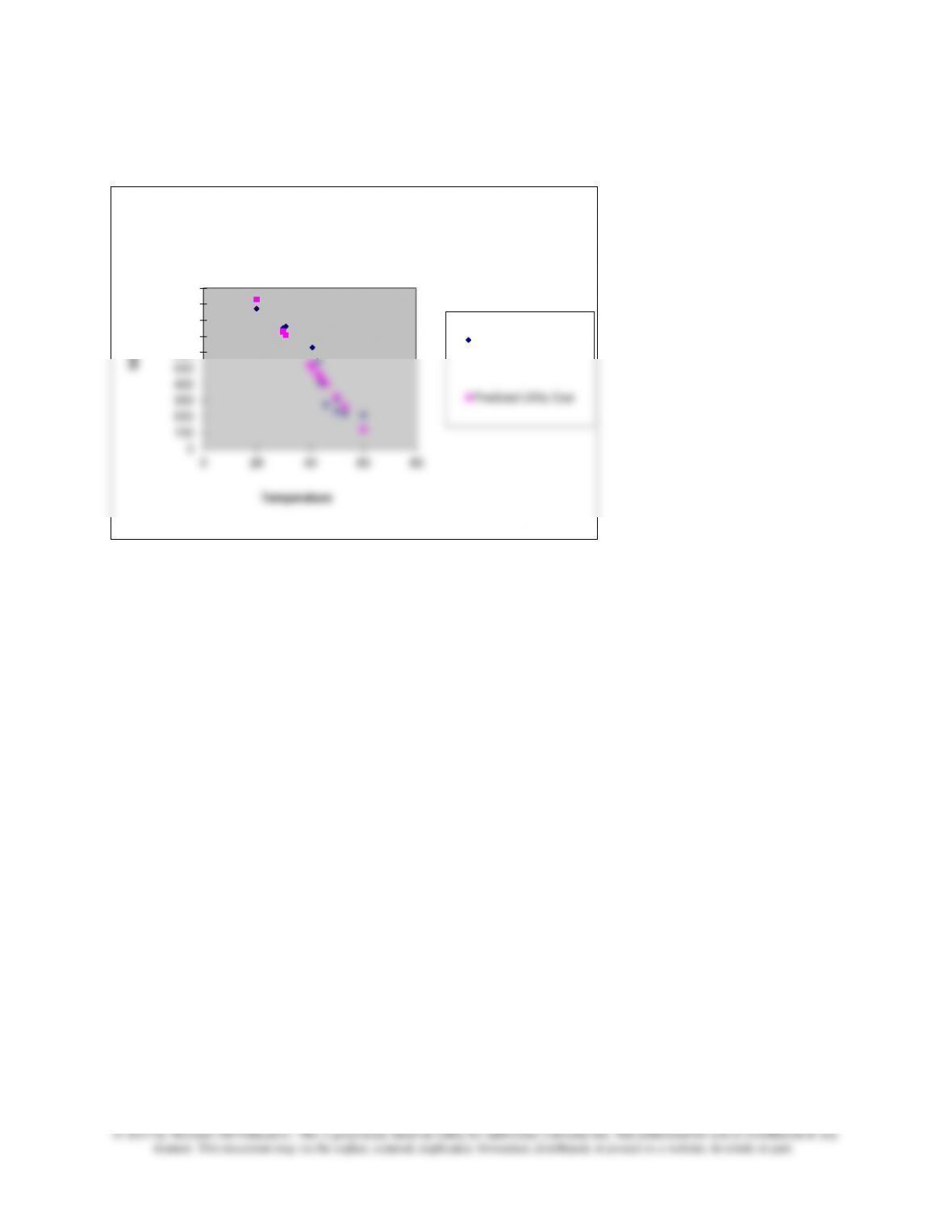
The cost/temperature relationship is shown in the Excel chart below:
0
100
200
300
400
500
600
700
800
900
1000
020 40 60 80
Utility Cost
Temperature
Temperature Line Fit Plot
Utility Cost
Predicted Utility Cost
Chapter 8 – Cost Estimation
8-37
8-45 Regression Analysis; Evaluating Regression Equations (20 min)
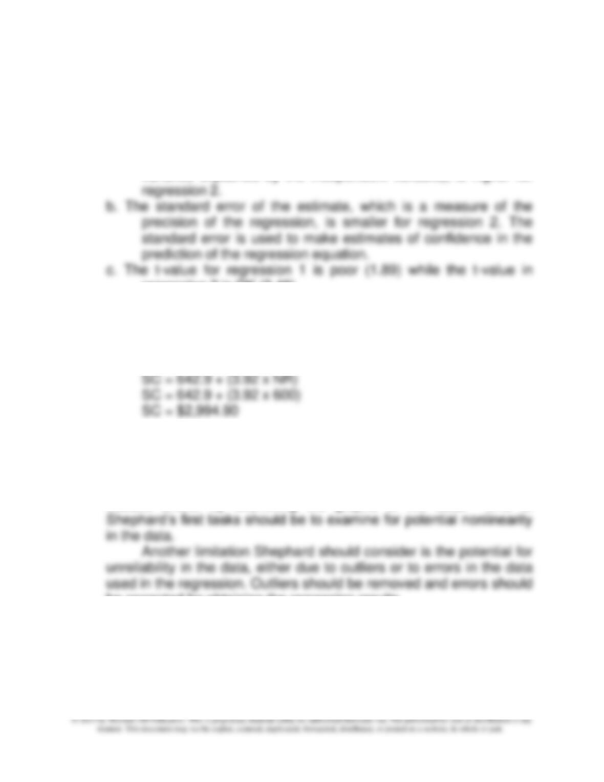
1. The Pilot Shop should adopt regression 2 to forecast total shipping
department costs for the following reasons:
a. R-squared, the coefficient of determination (the proportion of the
variance explained by the independent variable), is higher for
regression 2 is OK (3.46).
2. Since the number of orders to be shipped next week is given, the
appropriate estimation model is regression 2, and the total estimated
shipping cost is $2,994.90.
3. An important limitation of the regression we have chosen is that we
have not been able to assess the potential for nonlinearity in the
relationships among the variables. The presence of nonlinear
relationships can be assessed by examining the Durbin-Watson
statistic and/or by examining the graphs of the data. One of
be corrected for obtaining the regression results.
An additional limitation is that we are unable to assess the potential
for nonconstant error variance since we do not have a graph of the
data. Maynard should prepare a graph of the data and assess the
potential for nonlinearity.

8-38
8-45 (continued –1)
The global nature of the Pilot Shop’s operations adds another
limitation to the analysis. The purchasing and shipping costs will vary
with international business conditions and also with fluctuations in
Chapter 8 – Cost Estimation
8-46 Regression Analysis (20 min)
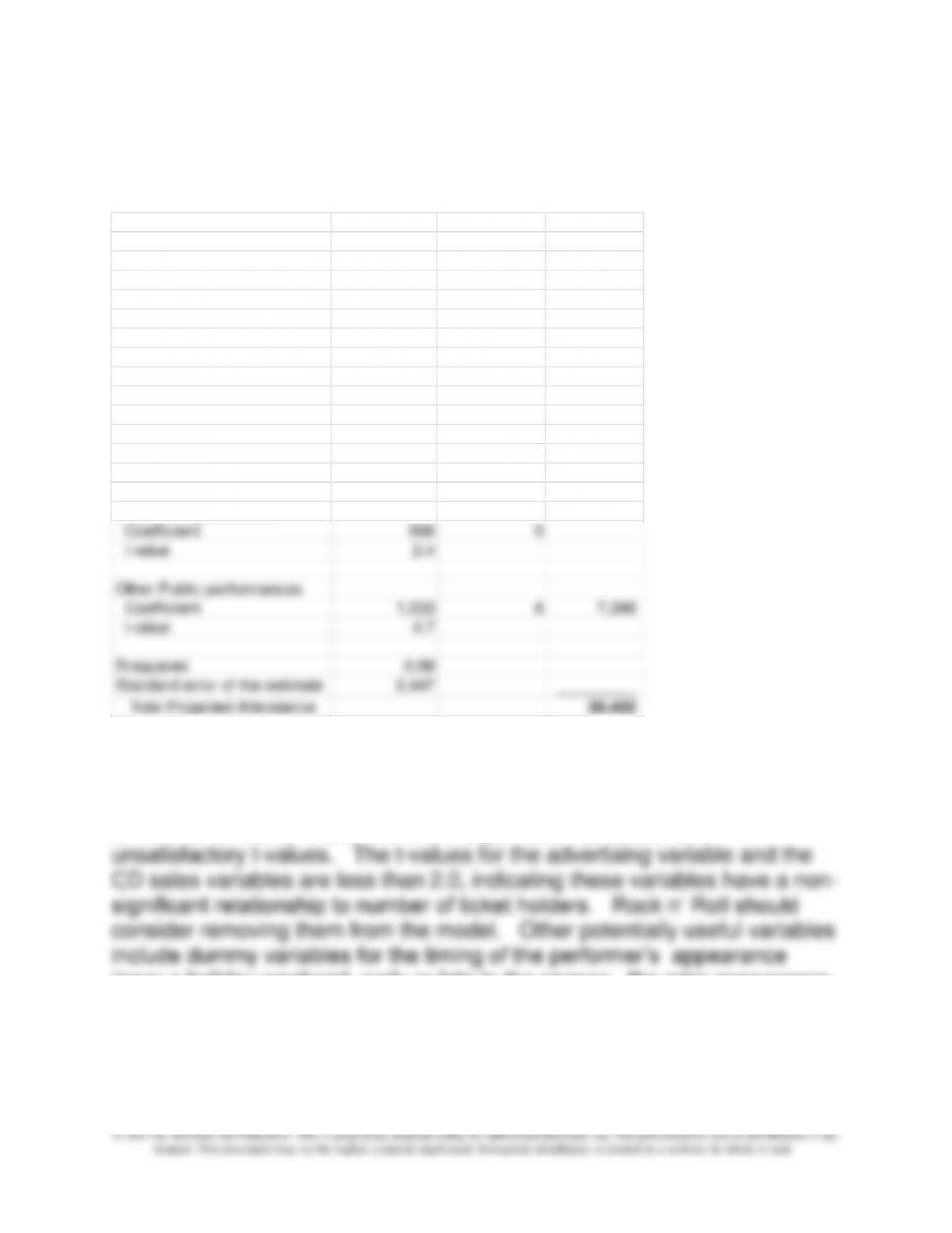
1.
The total projected attendance is 20,422, as determined below.
Independent Variables Results Example Totals
Regression intercept 1,224 1,224
Attendance at prior concert
Coefficient 3445 1 3,445
t-value 4.11
Spending on advertising
Coefficient 0.113 35,000 3,955
t-value 1.88
Performer’s CD sales
Coefficient 0.00044 10,000,000 4,400
t-value 1.22
Television appearances
Coefficient 898 0
t-value 2.4
Other Public performances
Coefficient 1,233 6 7,398
t-value 3.7
R-squared 0.88
Standard error of the estimate 2,447
Total Projected Attendance 20,422
2. The overall reliability of the regression, as measured by R-squared is
very good, at 88% and the standard error of the estimate, at 2,447 is
reasonably small, considering the level of predicted attendance, 20,422.
On the other hand, two of the five independent variables have
(near a holiday weekend, early or late in the season, the prior appearance
was on a rainy day, etc), and other variables related to the performer’s
popularity, such recent appearances in the print media, release of a new
8-40
8-47 Correlation Analysis (20 min)
1.
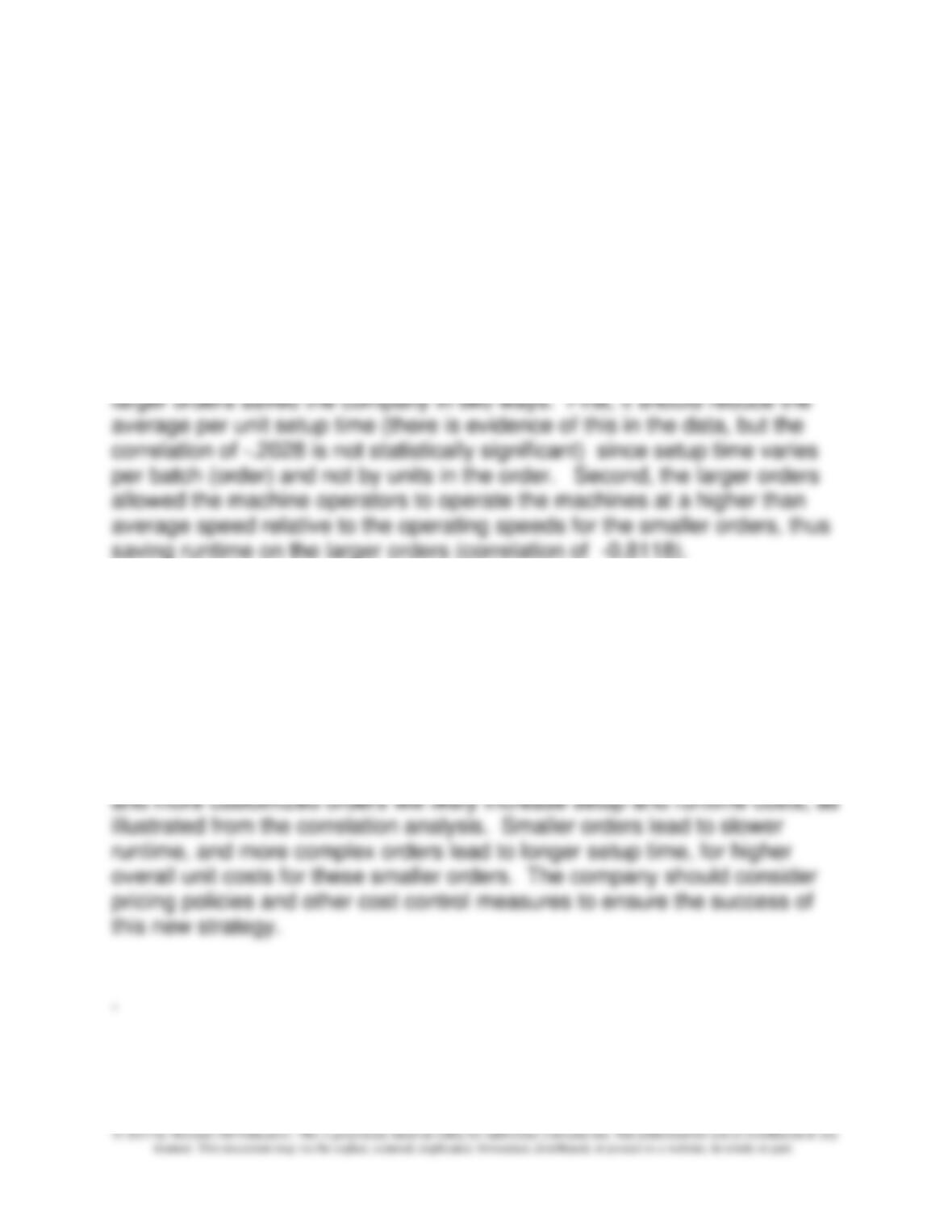
The correlation analysis shows that only one of the correlations is
significant at the .05 level – order size and runtime, and the relationship is
negative, or inverse. That is, the larger the order size, the smaller the
runtime per unit. Based on an actual company, this result is due to the fact
that the machine operators slowed the machine time at the start of each
order to ensure that the order was running properly before getting the
machine up to the normal runtime speed. The effect of this practice is that
Another informative aspect of the correlation analysis is to show the
positive (.459) and marginally significant (p< 0.10) relationship between
complexity and setup time per unit. This means that greater complexity
tends to increase setup time, an intuitive result.
2. The information above is particularly useful to PolyChem as it begin to
focus on smaller customers in order to find profitable alternatives to the
low-cost competition it now faces. The key point is that selling in smaller
Chapter 8 – Cost Estimation
8-41
8-48 Regression Analysis (20min)
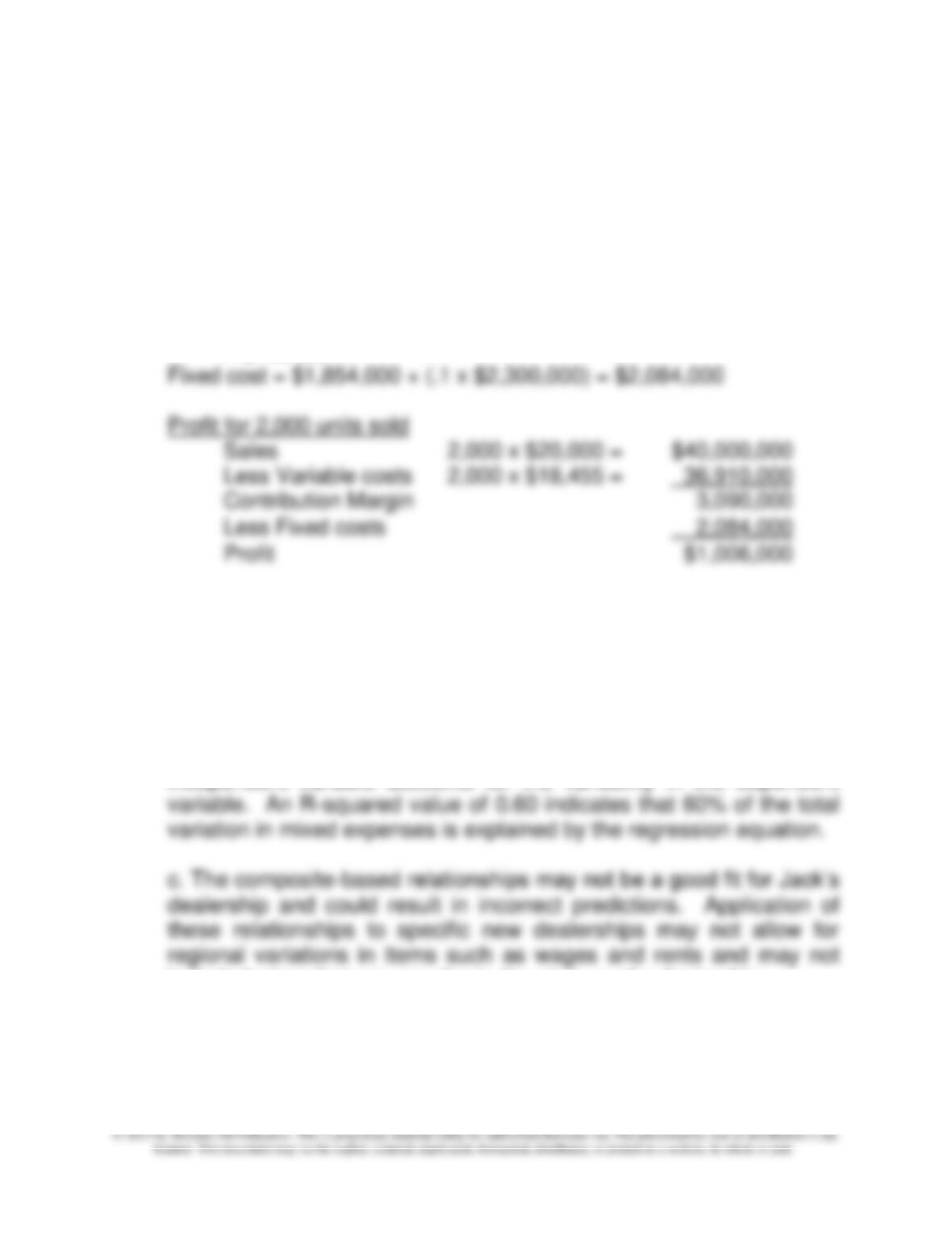
1. Assuming that all purchases of autos for resale (cost of goods
sold) represent variable costs
Price = $30,000,000/1,500 = $20,000
Variable cost per unit =
= [$862,500 + (.9 x $2,300,000) + $24,750,000] / 1,500
= $ 18,455
2.
a. The relevant range is the band or range of activity within which
specified cost relationships (behavioral assumptions) remain valid
and fixed costs remain fixed.
b. The R-squared value is a measure of the goodness of fit between
the independent and dependent variable, the extent to which the
independent variable accounts for the variability in the dependent
include factors that are peculiar to the start-up of a dealership.
d. The standard error of the estimate is the measure of precision of
the regression. The standard error of the estimate helps to determine
8-42
© 2013 by McGraw-Hill Education. This is proprietary material solely for authorized instructor use. Not authorized for sale or distribution in any
manner. This document may not be copied, scanned, duplicated, forwarded, distributed, or posted on a website, in whole or part.
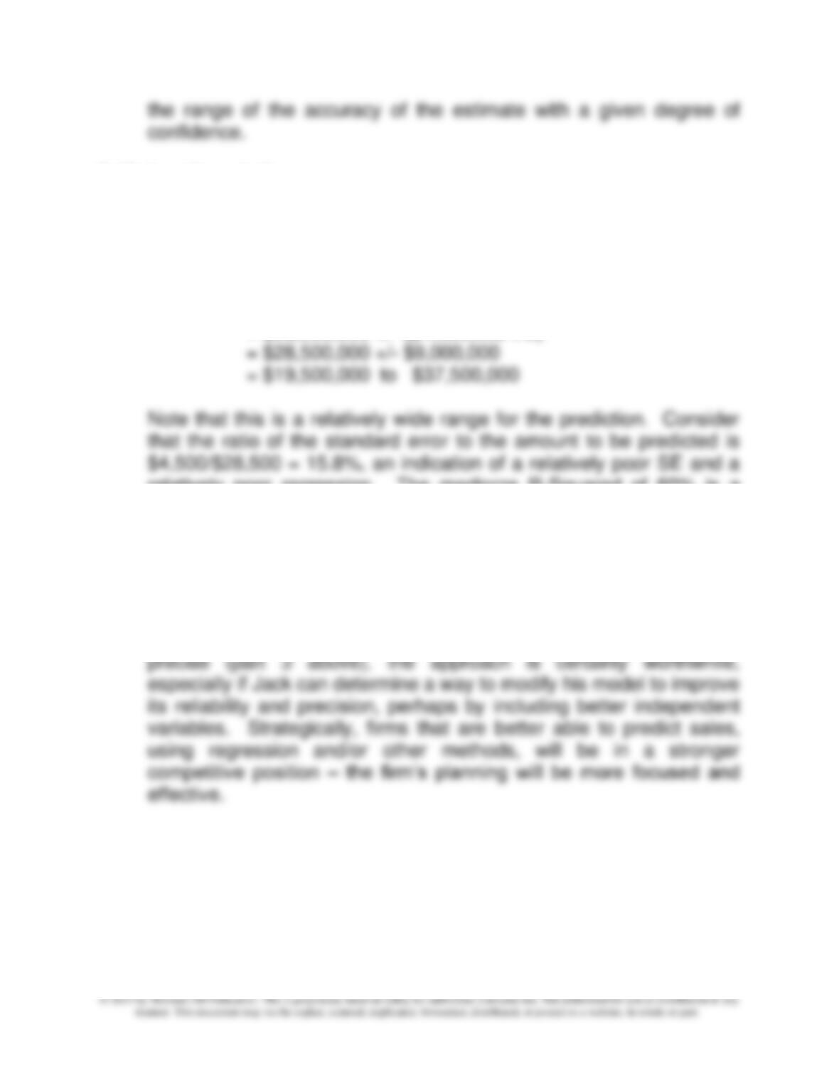
the range of the accuracy of the estimate with a given degree of
confidence.
8-48 (continued -1)
3. Using the regression equation that Jack Snyder developed, the
approximate range of sales that could occur during the year is
calculated below.
Range of sales = Sales +/- (Standard error x 2)
= $28,500,000 +/- ($4,500,000 x 2)
relatively poor regression. The mediocre R-Squared of 60% is a
further indication of the weakness of the model, and therefore of the
lack of precision of the predictions from the model.
4. A key issue for USMI is the risk of expanding its dealership
network. Regression analysis allows financial managers to make
predictions about the effect of the proposed expansion on sales and
profits. While Jack Snyder’s model is not particularly reliable or
Chapter 8 – Cost Estimation
8-43
8-49 Cost Estimation; High-Low Method, Regression Analysis (30min)
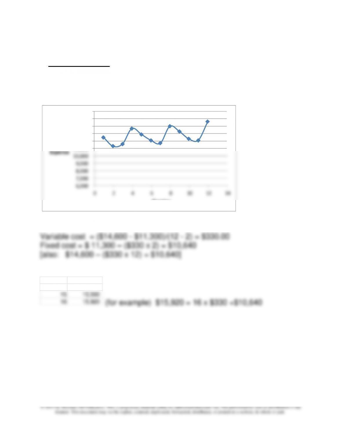
1. High-Low Method
An examination of the exhibit below indicates that representative high
and low points are the last and second data points, respectively, so
these points are used to develop the high-low estimate.
Quarterly Predictions are:
Because these predictions do not take into account all the seasonal
variation in the data, it is useful to consider the results for a regression
analysis, as shown below.
6,000
7,000
8,000
9,000
10,000
11,000
12,000
13,000
14,000
15,000
16,000
0 2 4 6 8 10 12 14
Return
Expense
Quarter
13 14,930$
14 15,260
15 15,590
16 15,920
8-44
8-49 (continued –1)
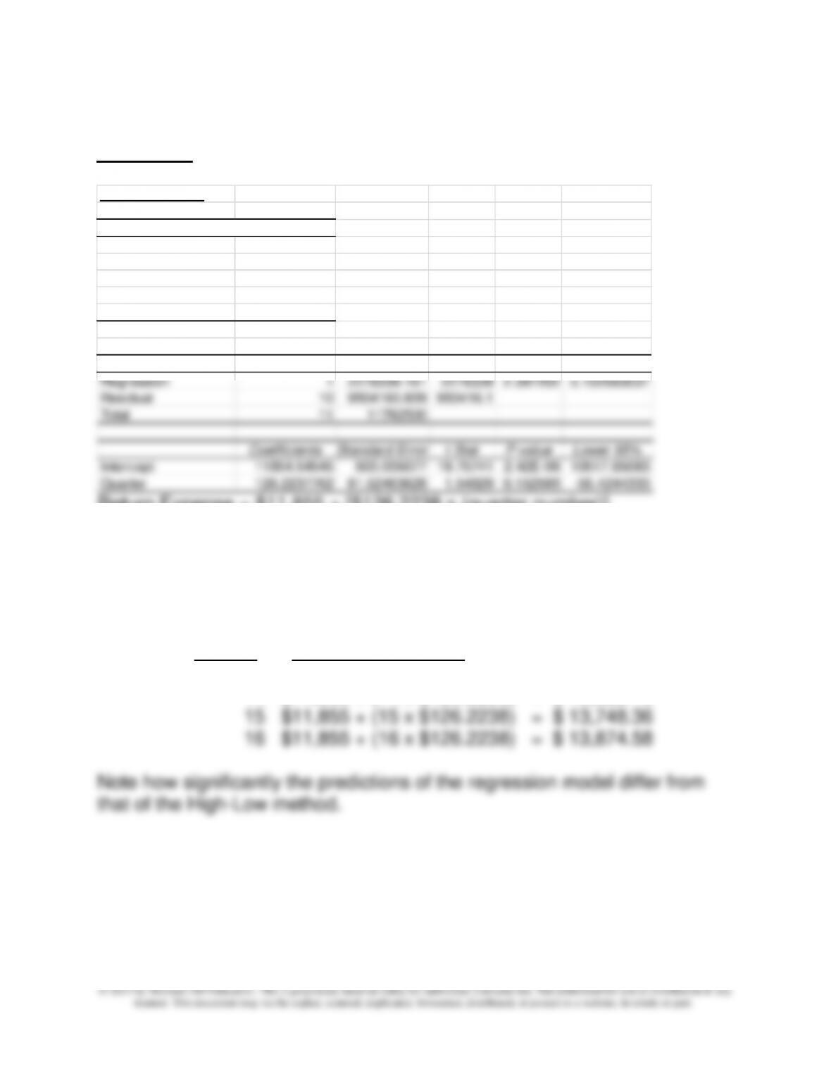
Regression
The regression equation from the spreadsheet (see below) is:
Regression One
Regression Statistics
Multiple R 0.439734422
R Square 0.193366362
Adjusted R Square 0.112702998
Standard Error 974.8928577
Observations 12
ANOVA
df SS MS F Significance F
Regression 1 2278339.161 2278339 2.397202 0.152593037
Residual 10 9504160.839 950416.1
Total 11 11782500
Coefficients
Standard Error
t Stat P-value Lower 95%
Intercept 11854.54545 600.005077 19.75741 2.42E-09 10517.65083
Quarter 126.2237762 81.52463628 1.54829 0.152593 -55.4244333
Return Expense = $11,855 + [$126.2238 x (quarter number)]
Predicted Expense for the next four quarters using regression analysis:
Quarter Regression Prediction
13 $11,855 + (13 x $126.2238) = $ 13,495.98
14 $11,855 + (14 x $126.2238) = $ 13,622.13
Chapter 8 – Cost Estimation
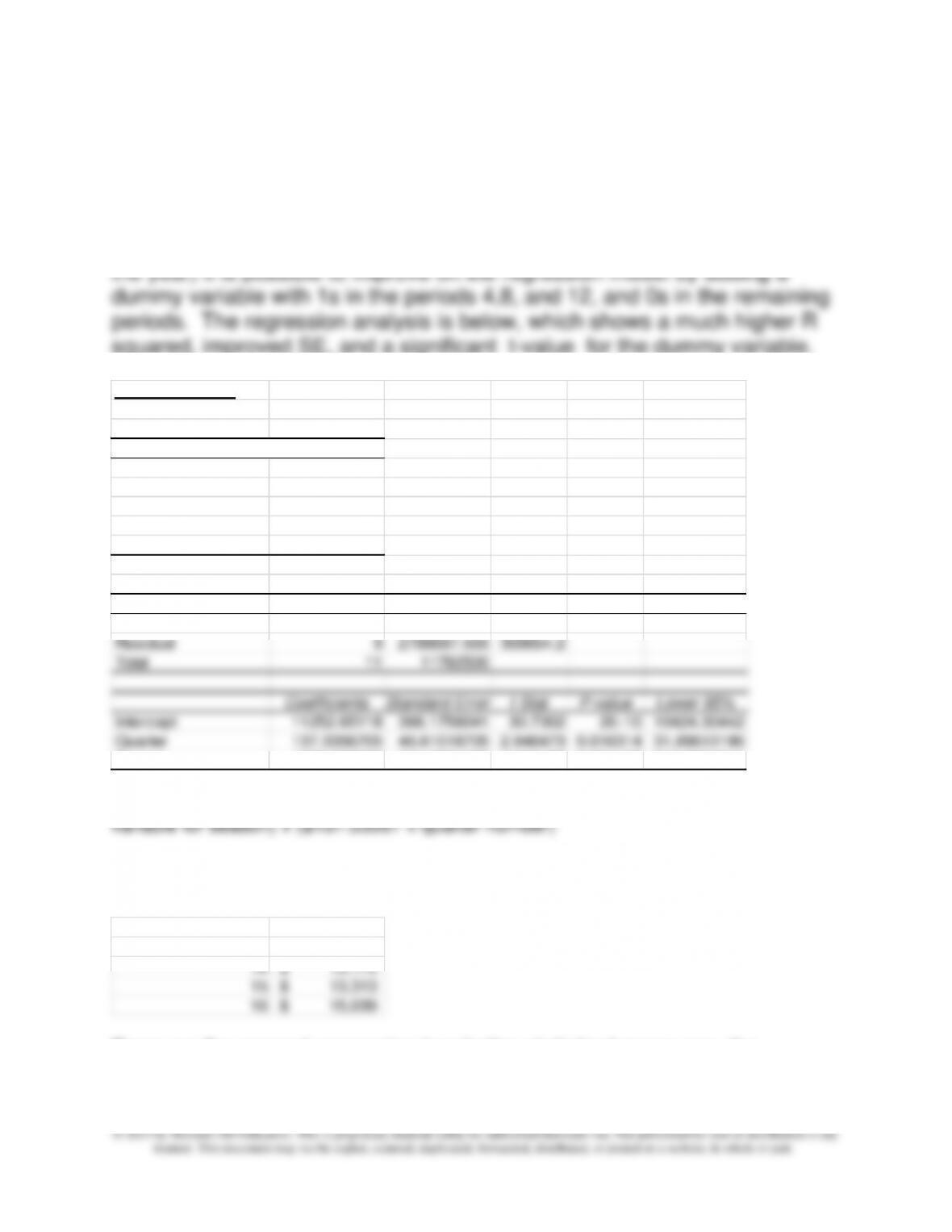
8-49 (continued –2)
At this point because of the relatively low R-squared, and the relatively low
t-value for the independent variable (note that the F value is not significant),
we consider a revision of the regression model. Since there is noticeable
seasonality in the data (higher for periods 1,4,8 and 12, the last quarters of
squared, improved SE, and a significant t-value for the dummy variable.
Regression Two
SUMMARY OUTPUT
Regression Statistics
Multiple R 0.873681599
R Square 0.763319537
Adjusted R Square 0.710723879
Standard Error 556.6454641
Observations 12
ANOVA
df SS MS F Significance F
Regression 2 8993812.445 4496906 14.51298 0.00152662
Residual 9 2788687.555 309854.2
Total 11 11782500
Coefficients
Standard Error
t Stat P-value Lower 95%
Intercept 11252.65118 366.1756041 30.7302 2E-10 10424.30442
Quarter 137.3356705 46.61018705 2.946473 0.016314 31.89610196
Season 1589.000876 341.3221703 4.655428 0.001193 816.8764841
This regression has the equation: Expense = $11,252.65118 + ($1,589.00876 x dummy
The regression predictions for the revised regression are as follows:
Quarterly Predictions
13 14,627$
14 13,175$
15 13,313$
16 15,039$
Because the second regression has better statistical measures, the
management accountant should rely on these predictions.