Unlock document.
This document is partially blurred.
Unlock all pages and 1 million more documents.
Get Access
8-16
8-35 Cost Estimation: High-Low method (15 min)
1.
Model to fit: Maintenance Expense = a + (b x M) (where M =
machine hours)
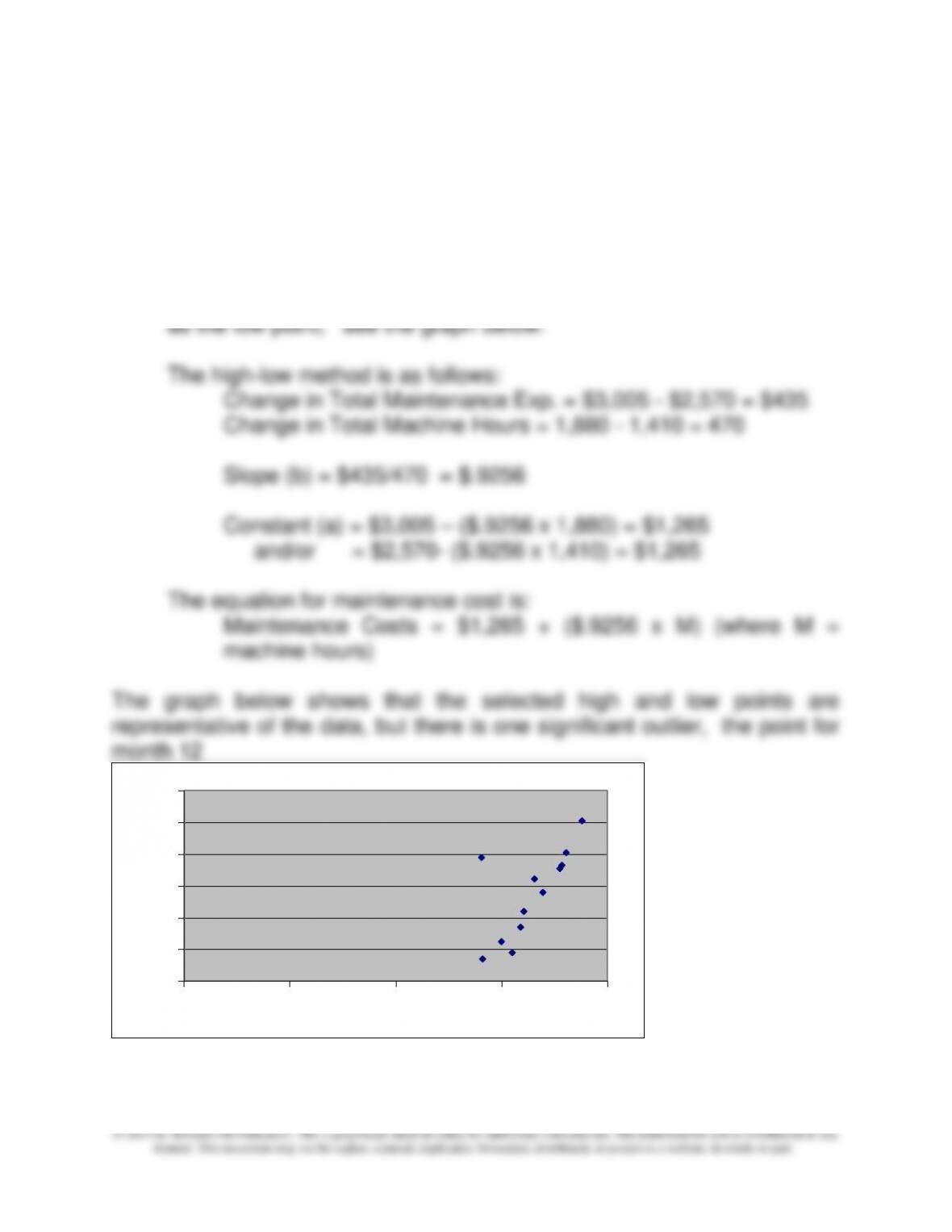
The highest and lowest points are months 6 and 10, respectively.
Note that the point for month 12 is an outlier, and should not be used
2500
2600
2700
2800
2900
3000
3100
0500 1000 1500 2000
8-17
8-35 (continued -1)
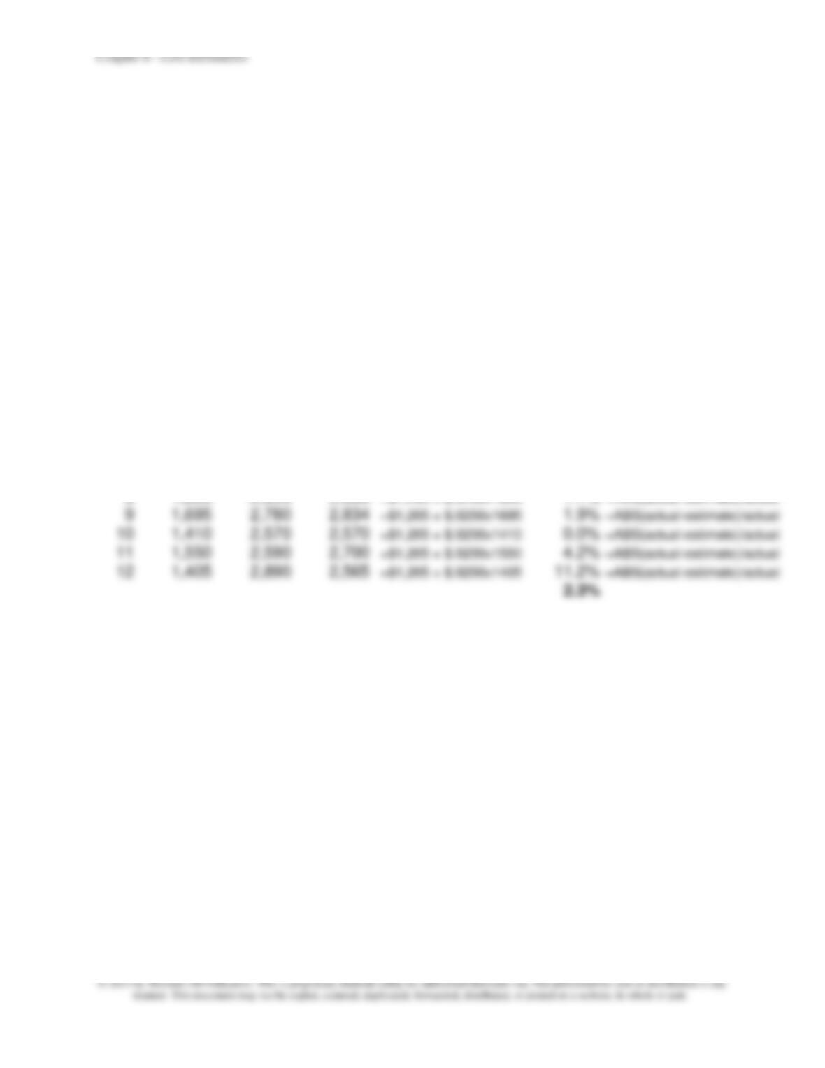
2. The mean absolute percentage error (MAPE) results are shown below.
MAPE is 2.3% for this 12 month period. Note that the outlier, point 12, has
a large MAPE. Overall, the MAPE is relatively low, due to the good fit of
the model to a set of data that is relatively linear.
Actual
Hours Expense
1 1,499 2,625 2,652 =$1,265 + $.9256x1499 1.0% =ABS(actual-estimate)/actual
2 1,590 2,670 2,737 =$1,265 + $.9256x1590 2.5% =ABS(actual-estimate)/actual
3 1,605 2,720 2,751 =$1,265 + $.9256x1605 1.1% =ABS(actual-estimate)/actual
4 1,655 2,822 2,797 =$1,265 + $.9256x1655 0.9% =ABS(actual-estimate)/actual
5 1,775 2,855 2,908 =$1,265 + $.9256x1775 1.9% =ABS(actual-estimate)/actual
6 1,880 3,005 3,005 =$1,265 + $.9256x1880 0.0% =ABS(actual-estimate)/actual
7 1,785 2,865 2,917 =$1,265 + $.9256x1785 1.8% =ABS(actual-estimate)/actual
8 1,805 2,905 2,936 =$1,265 + $.9256x1805 1.1% =ABS(actual-estimate)/actual
9 1,695 2,780 2,834 =$1,265 + $.9256x1695 1.9% =ABS(actual-estimate)/actual
10 1,410 2,570 2,570 =$1,265 + $.9256x1410 0.0% =ABS(actual-estimate)/actual
11 1,550 2,590 2,700 =$1,265 + $.9256x1550 4.2% =ABS(actual-estimate)/actual
12 1,405 2,890 2,565 =$1,265 + $.9256x1405 11.2% =ABS(actual-estimate)/actual
2.3%
Estimate
HiLo
MAPE
8-35 (continued -2)
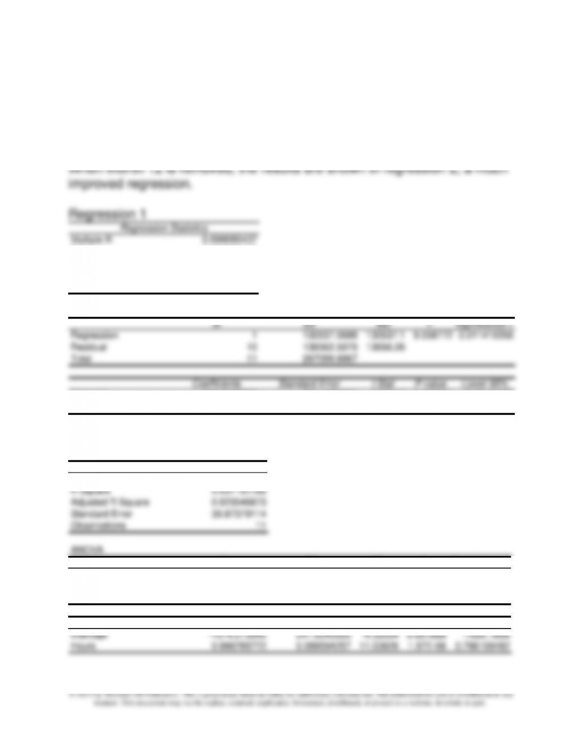
While not required for the exercise, a regression analysis on the data
produces the following results (regression 1). Note the significant
difference between the regression and the High-Low results. Also note the
relatively poor R-squared. This might be due to the outlier in month 12.
Residual 9 14309.27298 1589.919
8-19
8-36 Cost Estimation: High-Low method (30 min)
1.
Model to fit: Maintenance Expense = a + b x M (machine hours)
The highest and lowest points are months 5 and 10, respectively.
the high-low method is as follows:
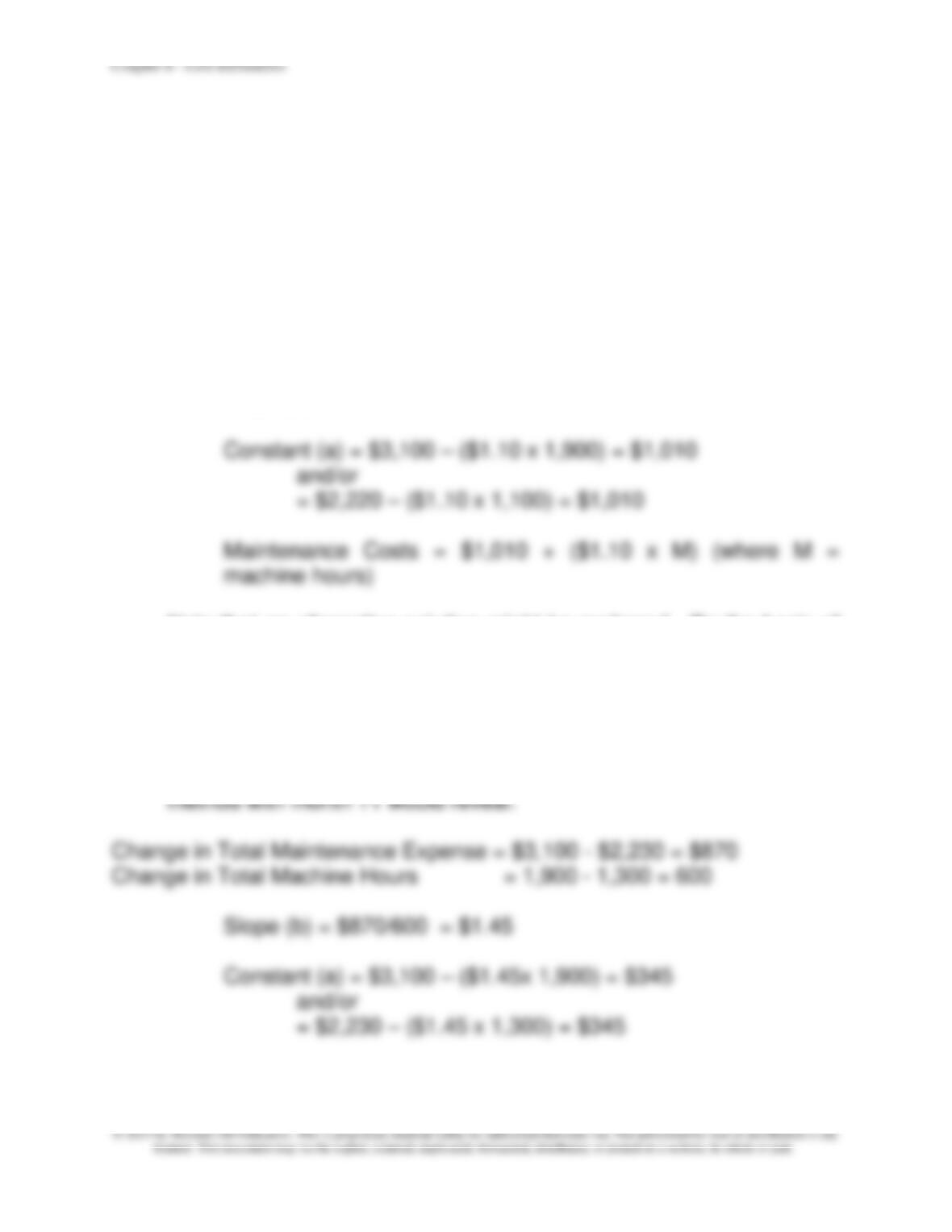
Change in Total Maintenance Expense = $3,100 - $2,220 = $880
Change in Total Machine Hours = 1,900 - 1,100 = 800
Slope (b) = $880/800 = $1.10
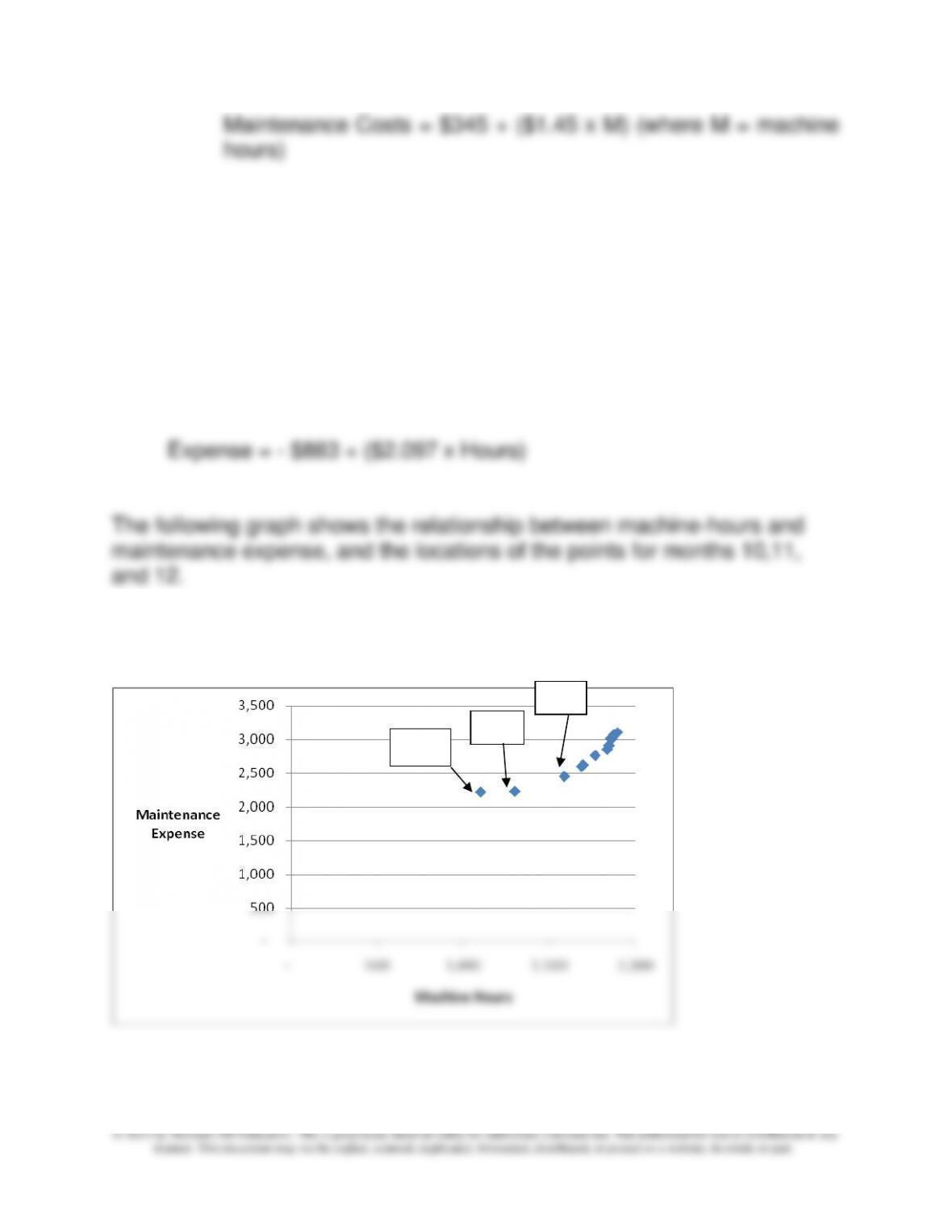
Note that an alternative solution might be preferred. On the basis of
a view of a graph of machine hours versus maintenance expense
(see below), it appears that the chosen lowest data point (month 10)
is not as representative of the relationships in the data as for month
11 (1,300 hours; $2,230). The point for month 10 is far to the left of
the remaining data points, while the point for month 11 is somewhat
closer to the remaining data points. A recalculation of the high-low
8-20
© 2013 by McGraw-Hill Education. This is proprietary material solely for authorized instructor use. Not authorized for sale or distribution in any
manner. This document may not be copied, scanned, duplicated, forwarded, distributed, or posted on a website, in whole or part.
Maintenance Costs = $345 + ($1.45 x M) (where M = machine
hours)
8-36 (continued-1)
The graph of expense versus hours showing the point for month 10 to be
an outlier (to the far left of the graph). One might also argue that the point
for month 11 is also an outlier and that the data for month 12 (1,590 hours
and $2,450) should be used instead. The model using month 12 as the
lowest month would be:
11
10
12
8-21
8-36 (continued -2)
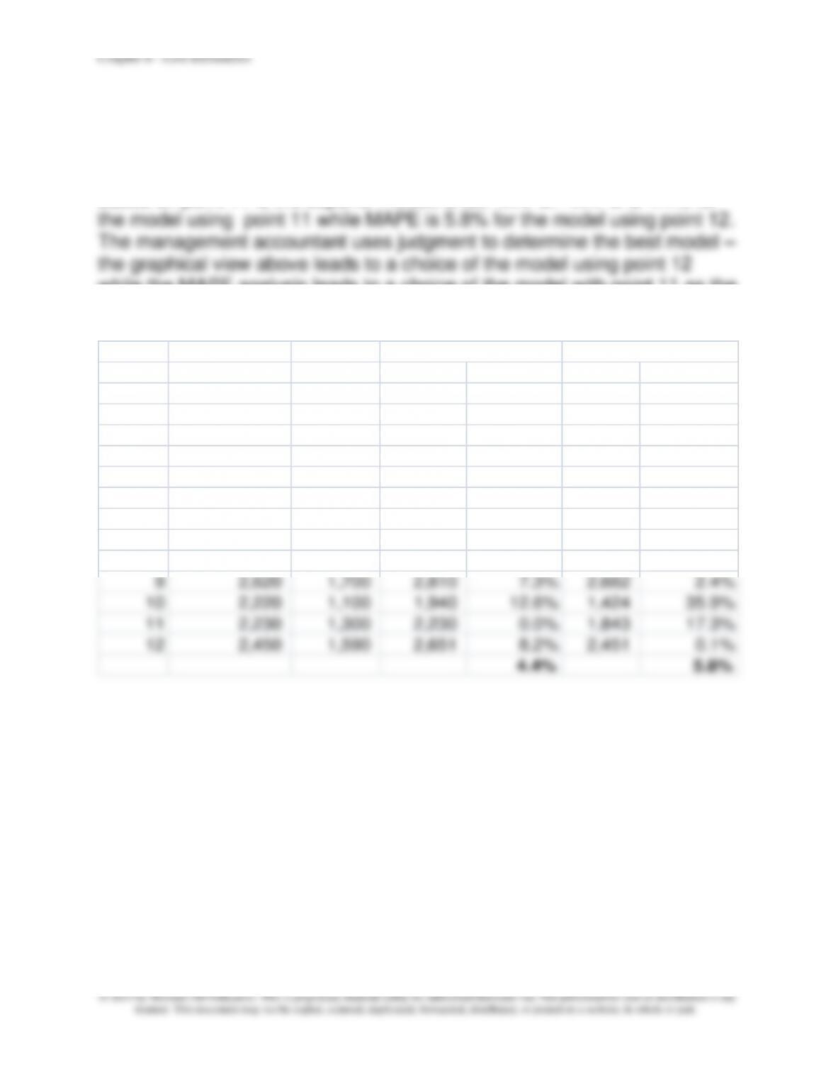
2. The calculation of the mean absolute percentage error (MAPE) for each
of the two high low models discussed in part one shows that the model
based on point 11 is the superior model, under MAPE. MAPE is 4.4% for
while the MAPE analysis leads to a choice of the model with point 11 as the
low point.
Maintenance Machine HiLo HiLo
Expense Hours Estimate MAPE Estimate MAPE
1 2,600 1,690 2,796 7.5% 2,661 2.3%
2 2,760 1,770 2,912 5.5% 2,829 2.5%
3 2,910 1,850 3,028 4.0% 2,996 3.0%
4 3,020 1,870 3,057 1.2% 3,038 0.6%
5 3,100 1,900 3,100 0.0% 3,101 0.0%
6 3,070 1,880 3,071 0.0% 3,059 0.3%
7 3,010 1,860 3,042 1.1% 3,017 0.2%
8 2,850 1,840 3,013 5.7% 2,975 4.4%
9 2,620 1,700 2,810 7.3% 2,682 2.4%
10 2,220 1,100 1,940 12.6% 1,424 35.9%
11 2,230 1,300 2,230 0.0% 1,843 17.3%
12 2,450 1,590 2,651 8.2% 2,451 0.1%
4.4% 5.8%
Point 11 - Low Point
Point 12 - Low Point
8-22
8-37 The Gompertz Equation; Learning Curves (20 min)
1.
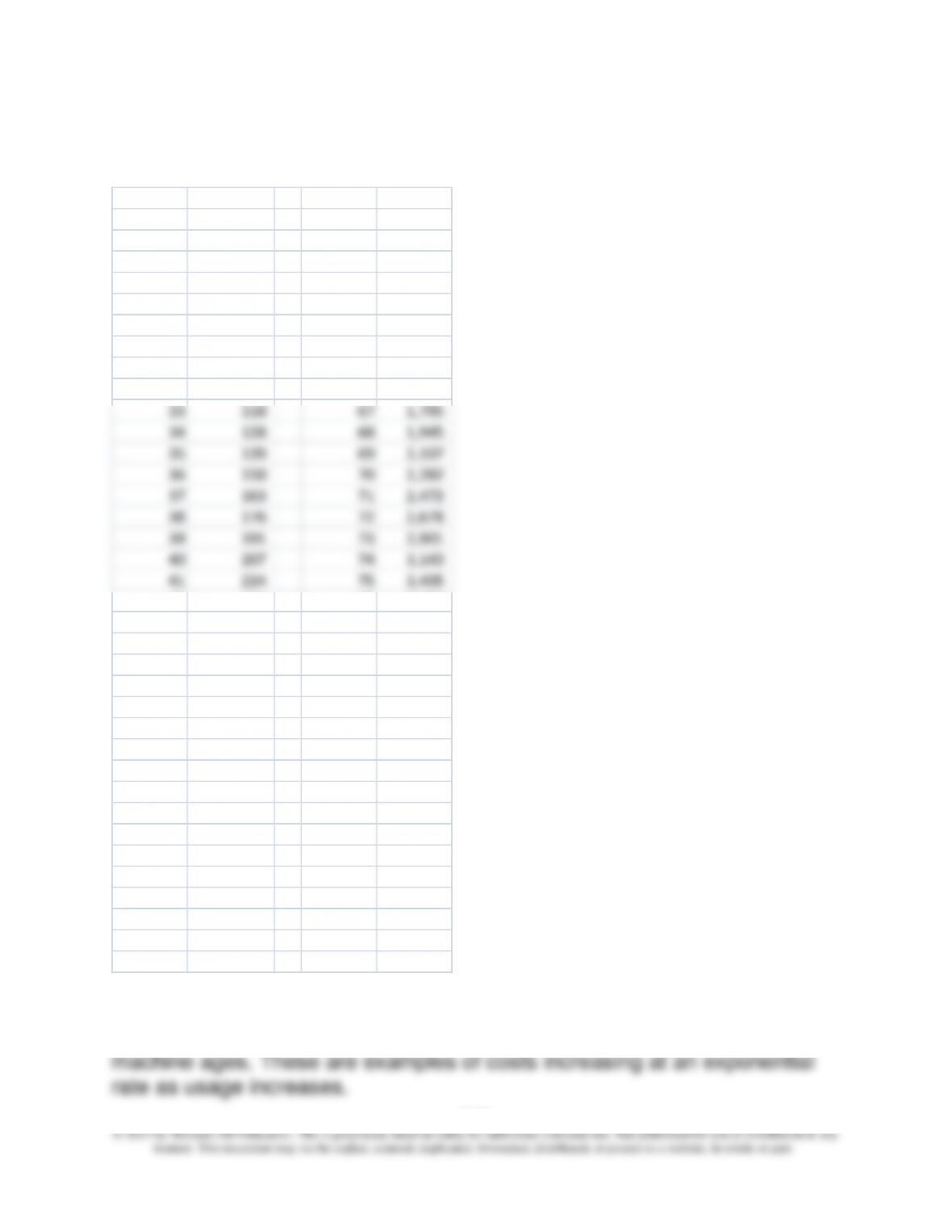
2. An exponential equation like the Gompertz equation could be used to
estimate the effect of employees working overtime on the production defect
rate, or it could be used to estimate the increase in maintenance cost as a
Mortality
Age Rate
25 62
26 68 60 1,026
27 73 61 1,111
28 79 62 1,203
29 86 63 1,304
30 93 64 1,412
31 101 65 1,530
32 109 66 1,657
33 118 67 1,795
34 128 68 1,945
35 139 69 2,107
36 150 70 2,282
37 163 71 2,472
38 176 72 2,678
39 191 73 2,901
40 207 74 3,143
41 224 75 3,405
42 243 76 3,689
43 263 77 3,996
44 285 78 4,329
54 635 88 9,633
55 687 89 10,436
56 745 90 11,305
57 807
58 874
59 947
Chapter 8 - Cost Estimation
8-23
8-38 Regression and Utility Rates; Sustainability (20 min)
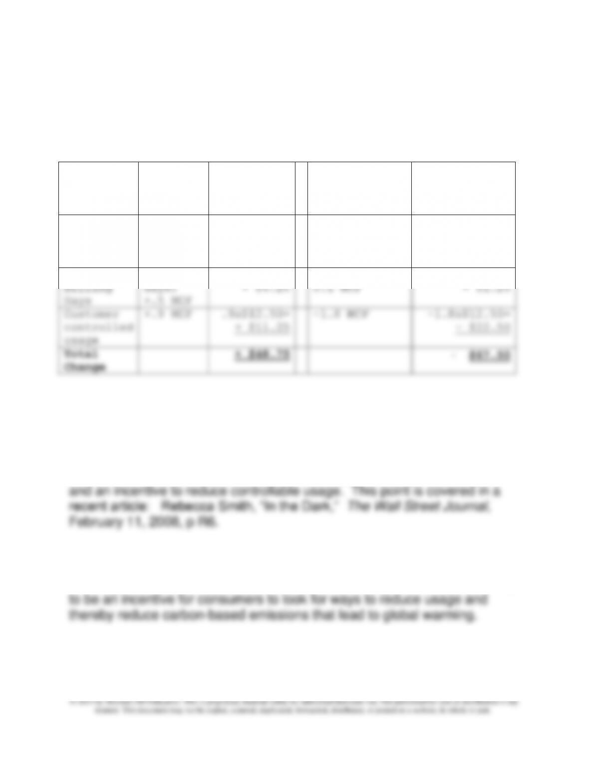
1. The calculations are as follows. The customer’s current bill was
$48.75 greater than last month’s bill, and $67.50 less than December
of the prior year.
Usage
Factors
Current
Month vs
Last
Month
$ Amount
Change
Current Month
vs Last
December
$ Amount
Change
Weather
3
degrees
cooler;
+2.5MCF
2.5x$12.50=
+ $31.25
8 degrees
warmer;
- 3.5MCF
-3.5x$12.50=
- $43.75
Number of
Billing
Days
5 more
days;
+.5 MCF
.5x$12.50=
+ $6.25
1 less day; -
0.1 MCF
-0.1x$12.50=
- $1.25
Customer
controlled
usage
+.9 MCF
.9x$12.50=
+ $11.25
-1.8 MCF
-1.8x$12.50=
- $22.50
Total
Change
+ $48.75
- $67.50
The above is based on an actual customer statement for a residence in
eastern Ohio.
The advantage of billing in this format is that the customer knows the cause
of the changes in the bill (related to weather and billing days) and also
knows the residual usage, or controllable usage, that can provide a basis
2.
The Dominion billing system facilitates environmental sustainability by
showing each user a “report card” of their recent usage. The result is likely
8-24
8-39 Interpreting Regression Results (10 min)
1. The estimated cost is:
$3,719 + (2 x $861) + (1 x $1,986) + (1 x $908) = $8,335
2. There are two dummy variables in this regression:
3. The model has a relatively low r squared of only 53%, but all three
independent variables have good t-values (>2.0). Looking at the t-values,
it appears that the strongest independent variable is the length of stay, and
the weakest is the use of laparoscope.
The exercise is based on information from: “Hospital Costs of Uterine
Artery Embolization…” by M Beinfeld, J. Bosch, and G Gazette, Academic
Radiology, Nov 9, No. 11, November 2002, pp 1300-1304.
8-25
8-40 Analysis of Regression Results (10 min)
1. The laparoscopic regression has the better regression result, with a
significantly higher R-squared and lower standard error for the number of
complications variable.
2. The t-value is the ratio of the coefficient to the standard error of the
independent variable. The t-values are shown below.
sample).
The t-values measure the statistical reliability of each independent
variable. A t-value of approximately 2 or larger indicates a statistically
reliable independent variable.
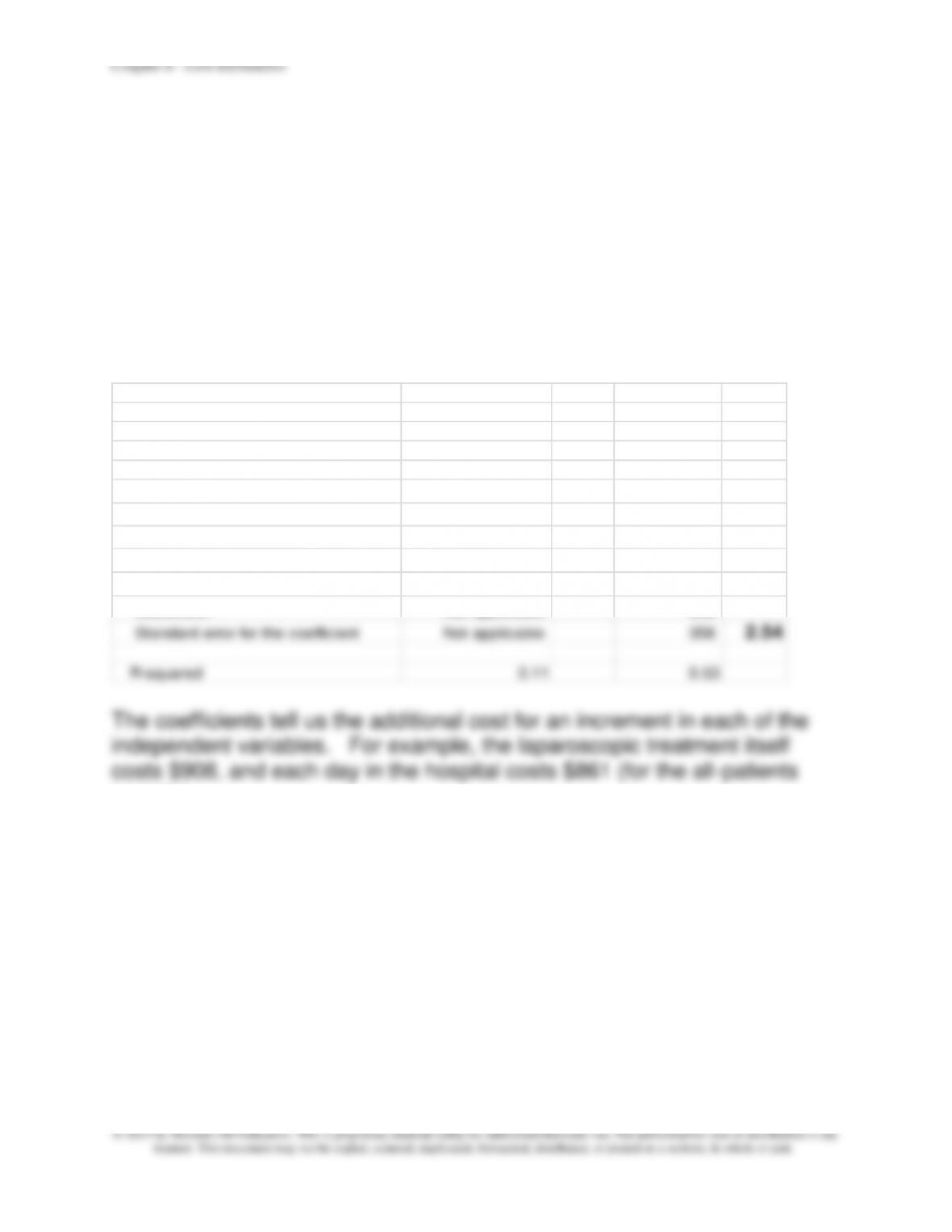
Not Laparoscopic All Patients
Coefficients for Independent Variables t-value t-value
Intercept 8,043$ 3,719$
Length of Stay
Coefficient Not significant 861
Standard error for the coefficient Not applicable 80 10.76
Number of Complications
Coefficient 3,393 1,986
Standard error for the coefficient 1,239 2.74 406 4.89
Laparascopic
Coefficient Not applicable 908
Standard error for the coefficient Not applicable 358 2.54
R-squared 0.11 0.53
8-26
8-41 Cost Estimation; High-Low Method (15 min)
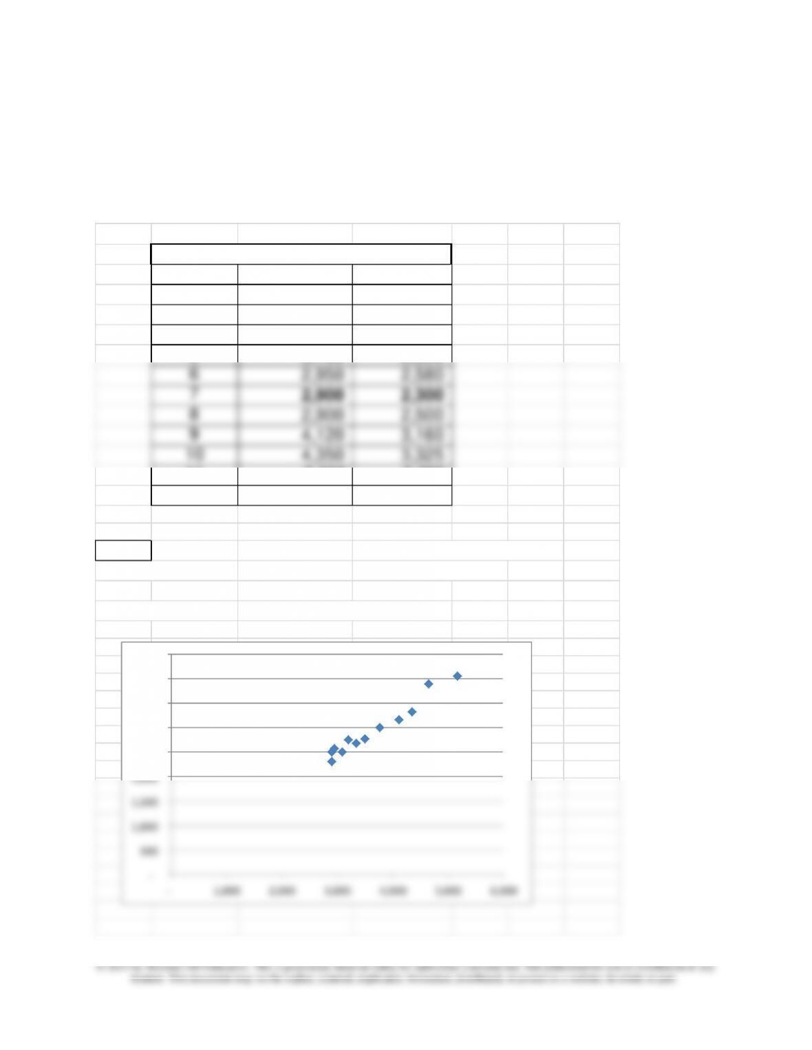
When months 3 and 7 are used for the high and low points respectively, the
High-Low method provides the cost equation: Cost = $190 + $1.30 x hours.
The graph below shows that the data is very linear; there are no outliers.
Month Maint. Cost Hours
13,210 2,750
24,650 3,900
35,175 4,050
43,350 2,690
53,100 2,500
62,950 2,580
72,900 2,300
82,900 2,500
94,120 3,160
10 4,350 3,325
11 3,500 2,780
12 3,775 3,000
Slope (b) = 1.30 =(5175-2900)/(4050-2300)
-90 =5175 - 1.30x4050
= $-90 + $1.30 x Hours
Constant (a) =
Cost equation
-
500
1,000
1,500
2,000
2,500
3,000
3,500
4,000
4,500
- 1,000 2,000 3,000 4,000 5,000 6,000
Chapter 8 - Cost Estimation
8-27
Exercise 8-41 (continued -1)
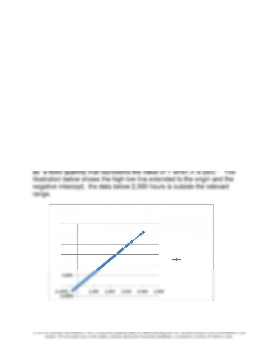
Note: the constant term in the solution is a negative number. This is a
good opportunity to explain to the students that a negative intercept term
can arise in a High-Low or a regression solution. The reason why is that
the relevant range for the independent variable is too far from the intercept,
so that the best-fitting High-Low line or regression line may have a negative
intercept. Chapter 3 included a discussion of the relevant range, with the
instruction that predictions of total cost should be limited to levels of the
independent variable that fall within the relevant range. This would be a
good time to remind the students of the concept of the relevant range and
how it applies to cost estimation. Wording to this effect is included on p
269 in the text.
This also reminds us that the value of a, the intercept, should not be
generally interpreted as fixed cost, especially when the relevant range of
the independent variable is far from the origin. The value of a is very useful
in developing the predicted cost from the cost estimation equation but
cannot be used to infer the level of fixed cost. Note that the text defines a
Negative intercepts also appear in exercises 35 and 36 (not in the solutions
but in commentary), and in Problems 50,54,and 56.
(1,000)
-
1,000
2,000
3,000
4,000
5,000
6,000
(1,000) - 1,000 2,000 3,000 4,000 5,000
Predicted Cost
Predicted Cost
8-28
PROBLEMS
8-42 Cost Estimation; High-Low Method (30 min)
1.
Analysis Based on Square Feet
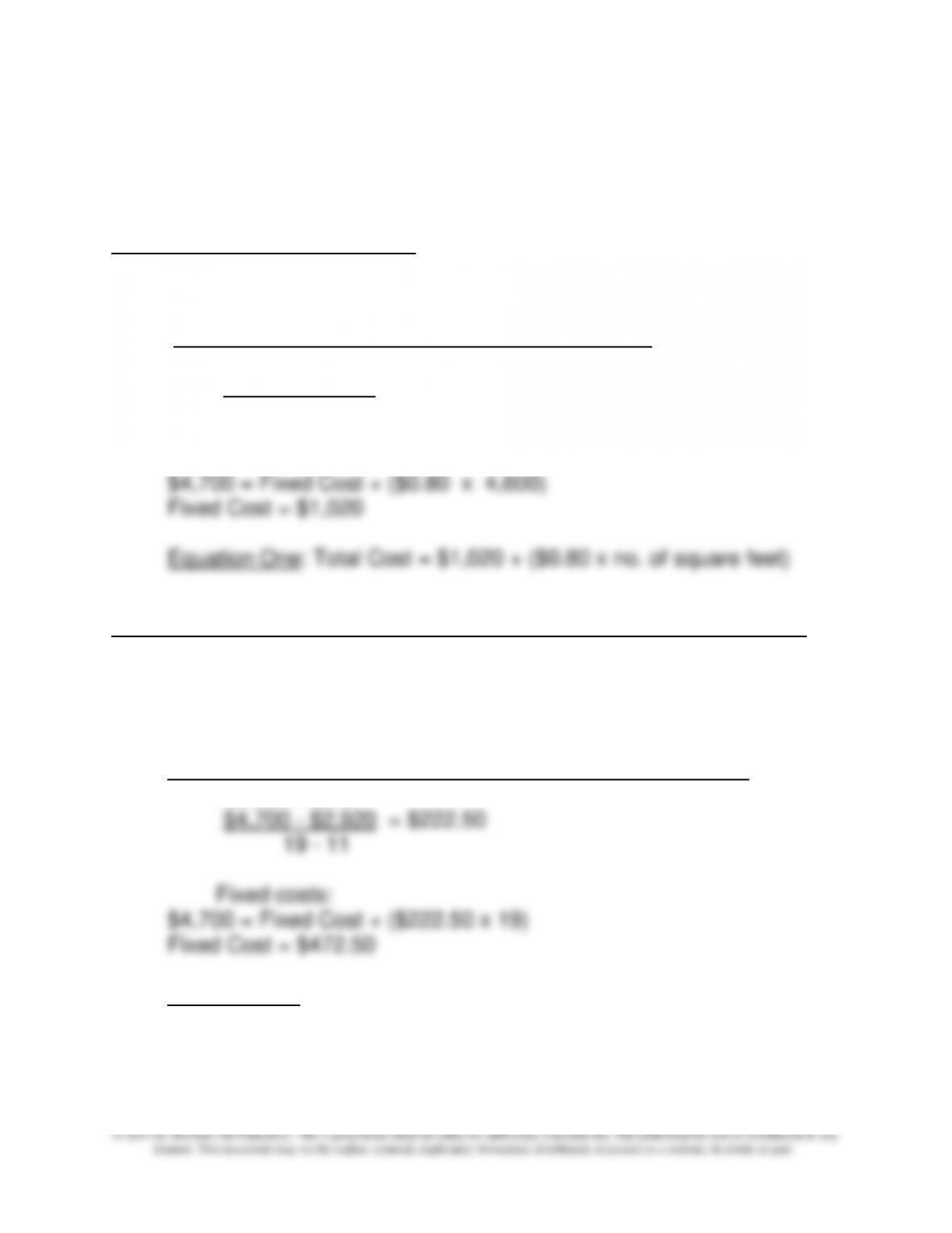
The high point is Home 5 and the low point is Home 7:
Cost equation using square feet as the cost driver:
Variable costs:
$4,700 - $2,920= $ 0.80
4,600 - 2,375
Fixed costs:
Analysis Based on Openings: (high is home 5, low is either home 7 or 9)
There are two choices for the Low point when using openings for the cost
driver (see charts below). At 11 openings (home 7) there is a cost of
$2,920 and at 10 openings (home 9) there is a cost of $2,945.
Cost equation using 11 openings as the cost driver (home 7):
Variable costs:
Equation Two: Total Cost = $472.50 + ($222.50 x no. of openings)
8-29
8-42 (continued -1)
Cost equation using 10 openings as the cost driver (home 9):
Variable costs:
$4,700 - $2,945= $195
19 - 10
Fixed costs:
$4,700 = Fixed Cost + ($195 x 19)
Fixed Cost = $995
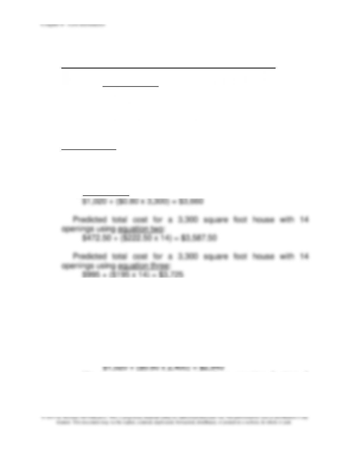
Equation Three: Total Cost = $995 + ($195 x no. of openings)
Predicted total cost for a 3,300 square foot house with 14 openings
using equation one:
There is no simple method to determine which prediction is best
when using the High-Low method. In contrast, regression provides
quantitative measures (R-squared, standard error, t-values,...) to help
assess which regression equation is best.
Predicted cost for a 2,400 square foot house with 8 openings, using
equation one:
We cannot predict with equation 2 or equation 3 since 8
openings are outside the relevant range, the range for which the high-
low equation was developed.
8-30
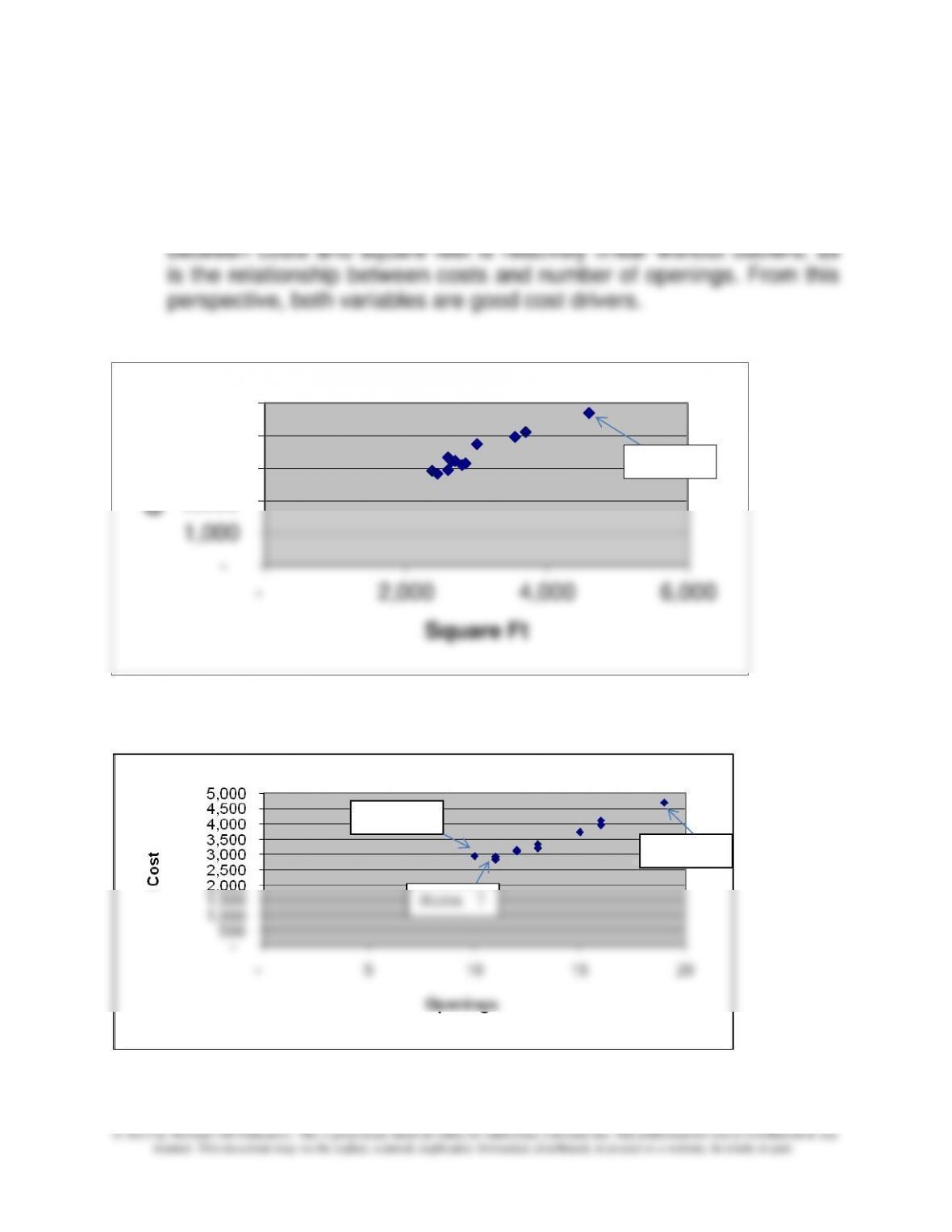
8-42 (continued -2)
2. See accompanying graphs, which show that the relationship
-
1,000
2,000
3,000
4,000
5,000
- 2,000 4,000 6,000
Cost
Square Ft
Home 9
Home 7
Home 5
Home 5


