
Chapter 8 – Cost Estimation
8-1
Chapter 8
Cost Estimation
Teaching Notes for Cases
8-1. High-Low Method and Regression Analysis
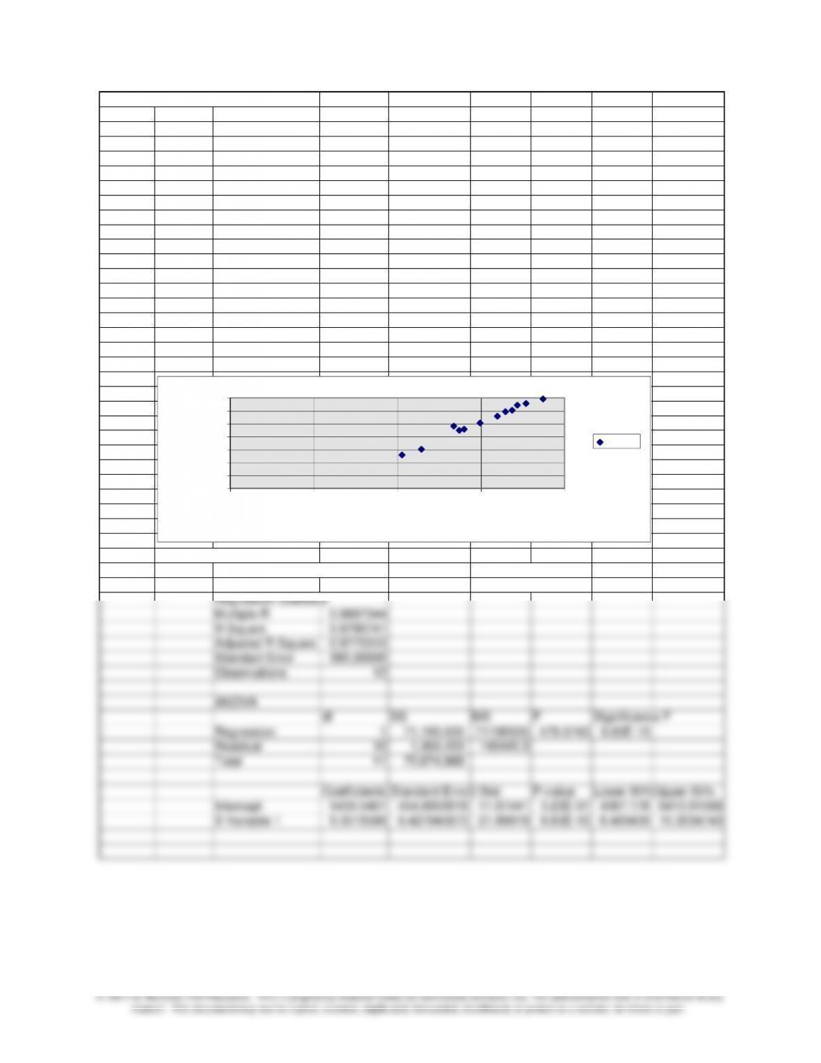
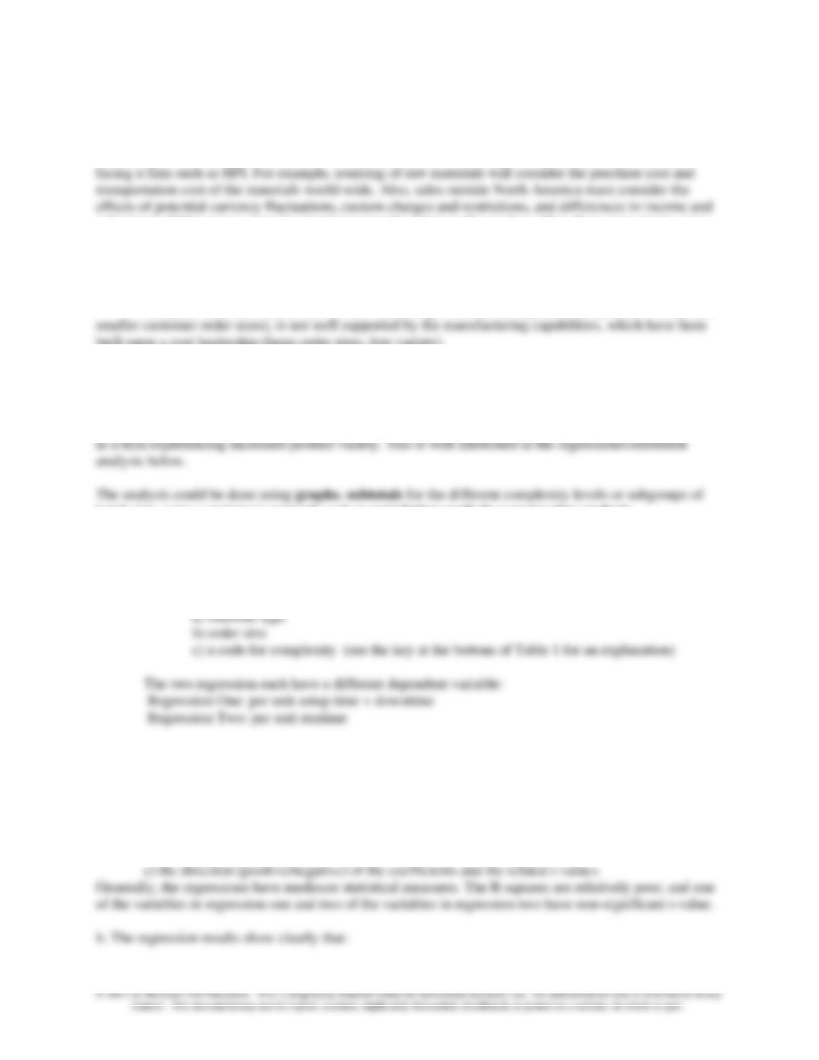
1, 2. The spreadsheet below shows the analysis of the Brenham Hospital data using both regression and
high-low methods. Before either method is applied, a scattergraph is prepared, as shown in the middle of
the spreadsheet; there are no apparent outliers or nonlinear patterns. The unit variable cost and fixed cost
for the high-low method are calculated, in the cells immediately below the figure, from the data in the
upper right hand corner of the spreadsheet⎯unit variable cost is $9.73 and fixed cost is $5,264. The
regression analysis is shown at the bottom of the spreadsheet⎯unit variable cost is similar to the high-
low results – $9.35; fixed cost is also similar to that of the high-low method, $5,400. We can be relatively
confident that these figures are at least approximately correct.
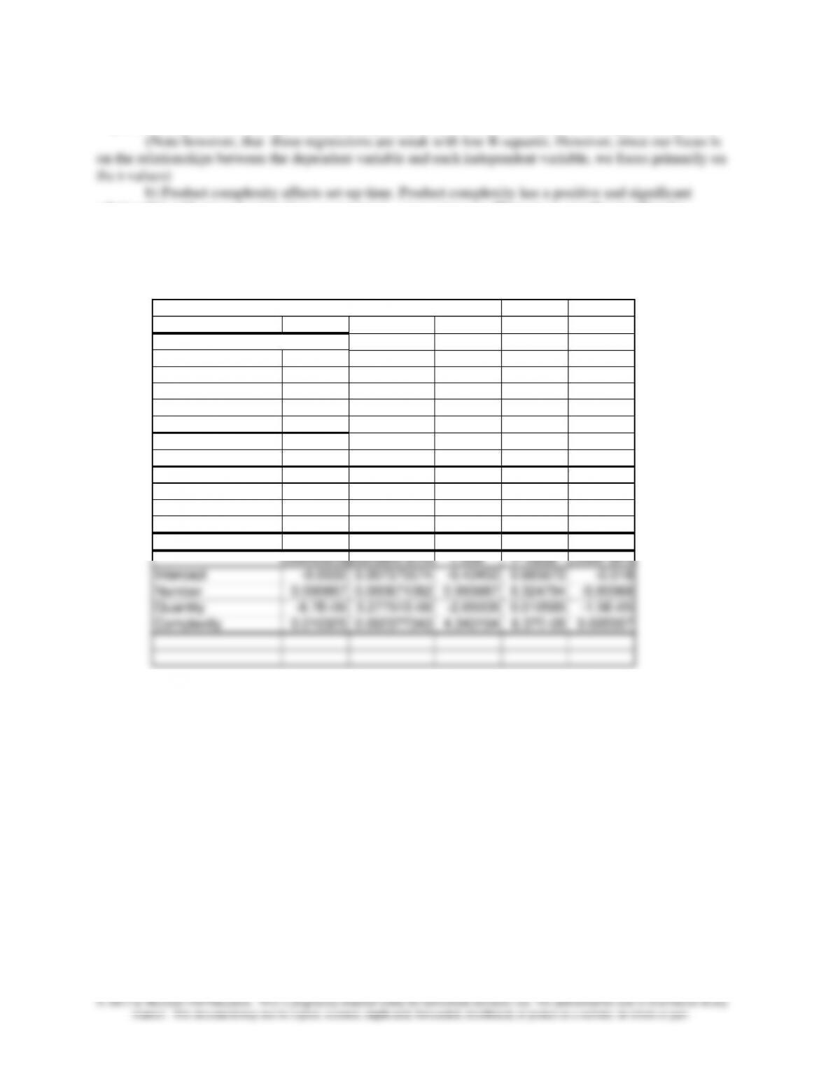
To evaluate the two methods, we examine the square error terms for each method. The error
terms for the high low method (squared) are shown in the top right portion of the spreadsheet⎯the total is
2,426,417. The total squared error for the regression is shown in the ANOVA table – 1,484,453. Since the
regression results are better, we would choose the regression model for the most accurate predictions.
3. Since unit variable cost is apparently less than $10, from both the regression and high-low results, and
since the fixed costs are unlikely to change (in fact the hospital says it plans to keep the dietician and
equipment), the best plan would be to keep the kitchen open, since the variable cost of the kitchen
(approximately $9.50) is less than the outside price of $11.50.
Chapter 8 – Cost Estimation
Brenham General Hospital
High Low
Other Food Total Patient Prediction
Dietician Staff Costs Maint. Equip. Cost Days Error
JAN 2,875 3,122 9,674 1,401 1,649 18,721 1,382 –
FEB 2,875 2,908 9,184 1,322 1,415 17,704 1,312 112,513
MAR 2,875 2,655 8,302 1,322 1,313 16,467 1,186 119,441
APR 2,875 2,600 7,084 1,288 1,105 14,952 1,012 27,693
MAY 2,875 2,433 6,398 1,200 1,089 13,995 914 28,634
JUN 2,875 2,083 4,338 1,133 1,011 11,440 604 86,535
JUL 2,875 1,809 3,612 1,093 900 10,289 516 –
AUG 2,875 2,322 6,275 1,122 1,112 13,706 896 80,063
SEP 2,875 1,434 6,734 1,235 1,103 13,381 962 1,563,944
OCT 2,875 2,700 9,002 1,302 1,300 17,179 1,286 368,783
NOV 2,875 2,798 8,456 1,300 1,442 16,871 1,208 24,277
DEC 2,875 2,600 7,798 1,322 1,396 15,991 1,114 14,534
34,500 29,464 86,857 15,040 14,835 180,696 12,392 2,426,417
Regression High Low:
SUMMARY OUTPUT Unit Variable cost 9.736721
Fixed Cost 5264.852
Regression Statistics
Multiple R 0.9897344
R Square 0.9795741
Adjusted R Square 0.9775315
Standard Error 385.28595
Observations 12
ANOVA
df SS MS F Significance F
Regression 1 71,190,535 71190535 479.5743 8.83E-10
Residual 10 1,484,453 148445.3
Total 11 72,674,988
Coefficients
Standard Error
t Stat P-value
Lower 95%
Upper 95%
–
200
400
600
800
1,000
1,200
1,400
– 5,000 10,000 15,000 20,000
Cost
Patient Days
Series1
8-3
8-2. Cost Estimation; Implementation
Background for the Case Answers:
Students will find it helpful if you go through the computations in the example in the case for job
1. This will also assure that they understand the nature of the adjustment that is being made. As you go
through the exhibit, emphasize that these adjustments are made only once a year even though many of the
jobs are in process for two and three years.
In the example in the case, the original cost estimate given on the first line is for reference only. It
is not used in the adjustment calculation. The second section calculates the costs incurred to date plus the
estimated costs to complete the job, yielding a new estimate for the total cost that will be required to
complete the job.
The third portion of the exhibit is the market value computation using the net realizable value less
a normal profit margin approach. The last line is the amount of the adjustment required to bring the
inventory carrying value (cost) down to lower of cost of market (LCM) .
For job 1, the LCM value of inventory will be ($2,100 + $373) – $572 = $1,901, while for job 2
the inventory value is $100 – $800 = $(700). Although this latter value may seem strange, the firm is
properly recognizing its loss on the job as soon as they become aware of it.
Next, you may wish to begin the discussion of the case by asking students to identify the major
problem areas that affect profitability. Then proceed to a discussion of the two specific questions.
The class discussion of the problem areas should reveal:
1. It appears that some jobs are accepted at unprofitable prices due to faulty cost-estimate
analysis (e.g., job 2 in the exhibit).
2. There is likely to be pressure put on the cost-estimate analysts by sales to keep estimates
low so as to generate additional sales. The analysts report to sales.
3. Feedback is slow. Problems are identified only when a job is complete or at the year-end
review of inventory. This makes it difficult to pinpoint responsibility and makes the taking
of timely corrective action nearly impossible.
4. The long production cycle exposes the firm to considerable risk due to inflation.
5. The large overhead rates suggest that the firm is not doing a very good job of tracing direct
costs to products. This, in turn, makes it difficult to have much confidence in the
cost/profitability figures.
Answers to Questions
1. (a) The cost-estimate analysts should not report to sales. It is likely that more realistic cost estimates
would result if this unit reported to a production manager.
In addition, a performance report should be devised for each cost-estimate analyst. This report
should routinely compare original cost estimates to actual costs incurred. If an analyst consistently over or
under estimates costs, corrective action can be taken. To be useful, such a report must be generated on a
an approach should help the analyst better estimate the actual costs that will be incurred to complete a job.
The controller should also undertake a study to determine the profits earned in the aftermarket
business relative to specific original equipment orders. Such a study would provide guidance on the
amount of the loss that can be justified on an original equipment order by the expected value of
aftermarket profits.
Chapter 8 – Cost Estimation
8-4
(b) Currently, the LCM review comes too late for effective control. The analysis should be made
much more frequently. A monthly analysis would provide the basis for the cost analyst’s performance
report and would also reveal any production problems on a more timely basis.
2. Because of the very large dollar investment in these products and the long in-process production times,
the carrying costs for inventory are substantial. Progress payments and advance payments shift a good
portion of the carrying costs (the cost of capital) to the customer.
With a fixed price contract the inflation risk is borne entirely by the company. Inserting estimates
of inflation in the contract puts risk on both the company and the customer for errors in the inflation
estimate. The use of escalation clauses is preferable because they hold the customer responsible for only
the actual inflation relative to the original cost estimate. It does not subject the customer to responsibility
for errors in cost or inflation estimates.
What the Firm Actually Did
The firm recognized the critical role played by the cost analyst. Errors here could doom the firm
to unprofitable contract even before work had begun. The firm changed the reporting relationship of the
analysts to report directly to the plant manager. In addition, the firm upgraded the quality of the analysts
by requiring more professional training.
The original cost analysis for each job became a standard. Monthly reports of actual costs
approved by the plant manager.
The firm now attempts to include progress billings in all contracts. If the customer refuses, a
charge for the cost of capital is now included in the original cost estimate. Coupled with the minimum
margin requirement, the cost of capital is now effectively included in each contract.
Escalation clauses are now required in all contracts which will require six or more months to
complete. Escalation clauses may be eliminated from a contract only with the plant manager’s approval.
Chapter 8 – Cost Estimation
8-5
8-3. Regression Analysis; Activity Based Costing; Strategy; International
Note to instructor: A variation on this case, shorter, with a focus on correlation analysis rather
than regression, is in the text, problem 8-47.
The firm is a large manufacturer of soap products for the hospitality industry. While the data is
real, the locations and descriptions are disguised. The firm has a goal of growth in sales, and has adopted
contemplating a significant expansion into the wholesale segment. A consequence of this strategy will be
an increased variety of products.
Teaching Objectives:
The case is very useful for an illustration of the potential application of ABC costing, because of
the firm’s diverse product line (packaging, soap fragrance, etc). A key result of the strategy conflict
opportunity to work with actual data in identifying cost driver relationships. Third, it illustrates the
complex inter-relationships among cost drivers.
The case was originally used in the manufacturing strategy course to illustrate the conflict
between manufacturing strategy (cost leadership) and marketing strategy (differentiation) in the case. The
case has been adapted to deal with cost drivers and strategic issues.
Main Points:
• Role of ABC Costing in a large packaging firm which is experiencing increased product
variety
• Use of Regression Analysis to Identify Cost Drivers
• Conflict of Manufacturing and Marketing Strategies
Discussion Questions:
1. What is HPI’s competitive strategy? How does HPI deal effectively with global competition in its
business?
HPI has built its business on differentiation, in the large hotel chain market. The attractive and
appealing soap products have developed this differentiation and given HPI a competitive advantage. As
hotel segment, and because of the related increase in excess manufacturing capacity.
Chapter 8 – Cost Estimation
8-6
An important feature of competition in the soap product business is cost leadership, as noted
above. By locating its plants near to its major markets and customers, HPI has located plants and
schedules production so as to minimize transportation costs. There are a large number of global issues
sales taxes. HPI’s excess capacity situation currently points to the need to either close some plants, or to
find new markets to keep current plants busy. This is in line with the firm’s current marketing initiatives.
2. What are the implications of the marketing and manufacturing initiatives undertaken by HPI?
The point should be made that the new marketing focus, involving increased product variety (and
built upon a cost leadership (large order sizes, low variety).
3. Using the data in Table 1 and appropriate methods of analysis such as regression or correlation
analysis, analyze the effect of order size and product variety on the productivity and cost structure of the
Paris plant.
The case is a good illustration of the value of ABC costing, to help measure product profitability
batch size, or by a statistical approach such as correlation analysis or regression analysis.
The solutions for the subtotal approach and graphical approach are not illustrated here but the
regression approach is shown below.
There are two regressions. Each of the two have the same three independent variables:
The students will likely make a variety of inferences from their individual analyses of the data.
After some discussion, make sure that the following points are made:
a. Assess the statistical measures for the regressions the students present, and/or for the regressions
attached. Make sure that the students understand the importance of evaluating the regressions:
a) the R-squared
b) the standard error
Chapter 8 – Cost Estimation
8-7
a) larger orders have lower per unit set up time and per unit runtime (i.e., better productivity)
⎯per both Regressions, the sign of the quantity independent variable is negative and significant (p<.05)
relationship with per unit setup time, as expected – regression one. There is no significant effect for
regression two.
Regression One
Dependent Variable: Per unit set-up time plus downtime
Regression Statistics
Multiple R 0.603189
R Square 0.363837
Adjusted R Square 0.327828
Standard Error 0.014407
Observations 57
ANOVA
df SS MS F
Significance
Regression 3 0.006291226 0.002097 10.10399 2.28E-05
Residual 53 0.011000104 0.000208
Total 56 0.01729133
Coefficients
Standard Error
t Stat P-value
Lower 95%
Intercept -0.0032 0.007375574 -0.43452 0.665672 -0.018
Number 0.000667 0.000671082 0.993887 0.324794 -0.00068
Quantity -8.7E-06 3.27751E-06 -2.65008 0.010585 -1.5E-05
Complexity 0.010325 0.002377343 4.343194 6.37E-05 0.005557
Chapter 8 – Cost Estimation
8-8
Regression Two
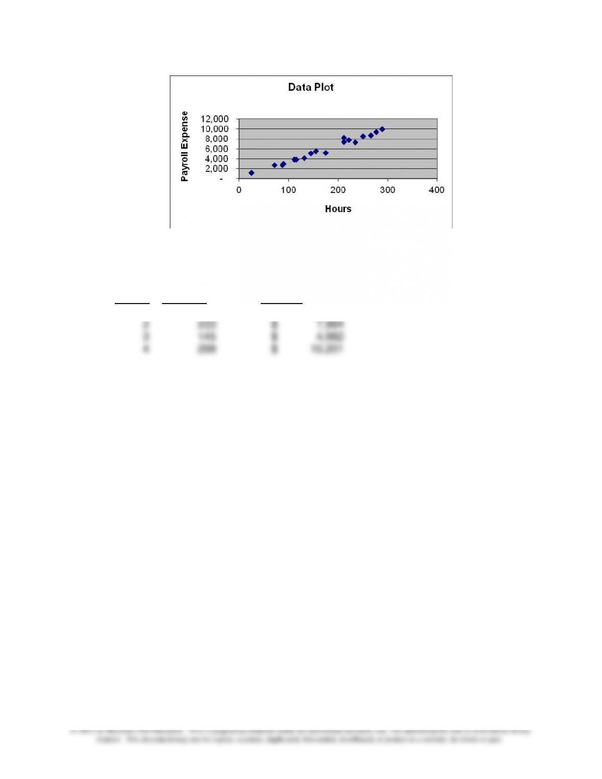
8-4 Custom Photography
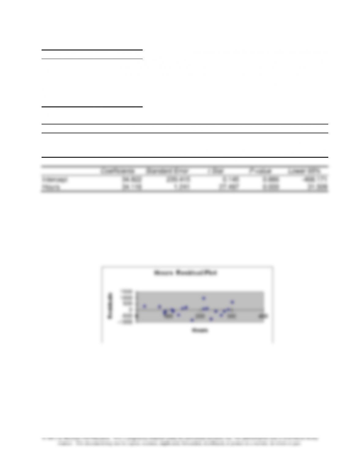
1. The Excel regression analysis for Custom Photography is shown below. Note that all the statistical
measures are excellent. The R-squared is very high, the standard error of the estimate is relatively low at
431/6,046 = 7% of the mean of the dependent variable and the t value of the independent variable is very
significant at t = 27.5.
The regression equation to predict payroll expense is:
Dependent Variable: Per unit runtime
Regression Statistics
Multiple R 0.58985361
R Square 0.34792728
Adjusted R Squa
0.31101751
Standard Error 0.0034273
Observations 57
ANOVA
df SS MS F
Significance F
Regression 3 0.00033218 0.00011073 9.4264263 4.304E-05
Residual 53 0.00062256 1.1746E-05
Total 56 0.00095474
Coefficients
Standard Error
t Stat P-value Lower 95%
Intercept 0.04555712 0.00175464 25.9638504 8.209E-32 0.0420378
Number 2.3785E-05 0.00015965 0.14898304 0.8821325 -0.0002964
Quantity -4.096E-06 7.7971E-07 -5.25336231 2.705E-06 -5.66E-06
Complexity -0.0008911 0.00056557 -1.5755149 0.1210886 -0.0020254
Chapter 8 – Cost Estimation
8-9
Regression Statistics
Multiple R
0.988
R Square
0.977
Adjusted R
Square
0.975
Standard Error
431.538
Observations
20
ANOVA
df
SS
MS
F
Significance F
Regression
1
140804738.725
140804738.725
756.101
0.000
Residual
18
3352047.475
186224.860
Total
19
144156786.200
Coefficients
Standard Error
t Stat
P-value
Lower 95%
Intercept
34.822
239.415
0.145
0.886
-468.171
Hours
34.116
1.241
27.497
0.000
31.509
Chapter 8 – Cost Estimation
8-10
2. Using the equation above, Payroll Expense = $34.82 + $34.12 x hours, predicted payroll is obtained as
follows:
Hours per
Predicted Payroll
Qtr No.
Qtr, 2002
Expense
1
188
$ 6,449
2
233
$ 7,984
3
145
$ 4,982
4
298
$ 10,201