
Chapter 8 – Cost Estimation
8-11
Case 8-5 Predicting the Effect of Poverty on High School Graduation Rate
High School graduation rates are a key measure of economic development and potential for economic
growth. The data below show the graduation rates and the percentage of children in poverty for each of
the states in the U.S. The graduation rate is for the school year 2004-2005 and the poverty data is for
2007. The data is from the U.S. Census Bureau and is reported in the November 24, 2008 issue of
Business Week, p 15.
Required:
1. Use regression analysis to answer the question whether there might be a causal relationship
between poverty level and graduation rates.
2. Critically examine the regression results you have developed. Include in your answer a
consideration of the data used and a consideration of potential additional variables that could be
used to predict graduation rates.
Chapter 8 – Cost Estimation
8-12
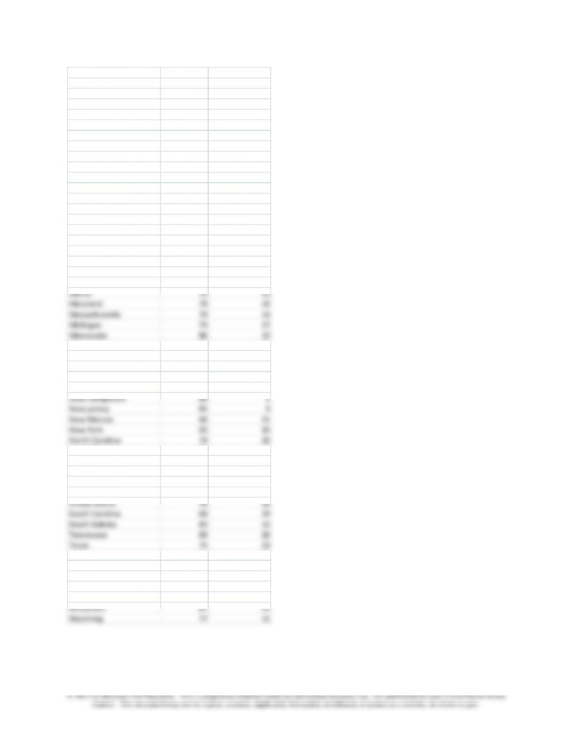
Graduation % of Children in
Rate (%) Poverty
Alabama 68 21
Alaska 64 8
Arizona 85 20
Arkansas 76 21
California 75 18
Colorado 77 14
Connecticut 81 10
Delaware 73 13
District of Columbia 73 33
Florida 65 16
Georgia 62 20
Hawaii 75 9
Idaho 81 11
Illinois 79 15
Indiana 74 17
Iowa 87 14
Kansas 79 18
Kentucky 76 22
Lousiana 64 24
Maine 79 13
Maryland 79 10
Massachusetts 79 13
Michigan 73 17
Minnesota 86 10
Mississippi 63 31
Missouri 81 19
Montana 81 17
Nebraska 88 13
Nevada 56 13
New Hampshire 80 5
New jersey 85 9
Ohio 80 18
Oklahoma 77 20
Oregon 76 16
Pennsylvania 83 16
Rhode Island 78 16
South Carolina 60 19
Vermont 87 7
Virginia 80 13
Washington 75 10
West Virginia 77 22
Wisconsin 87 15
Wyoming 77 11
Chapter 8 – Cost Estimation
Regression Analysis
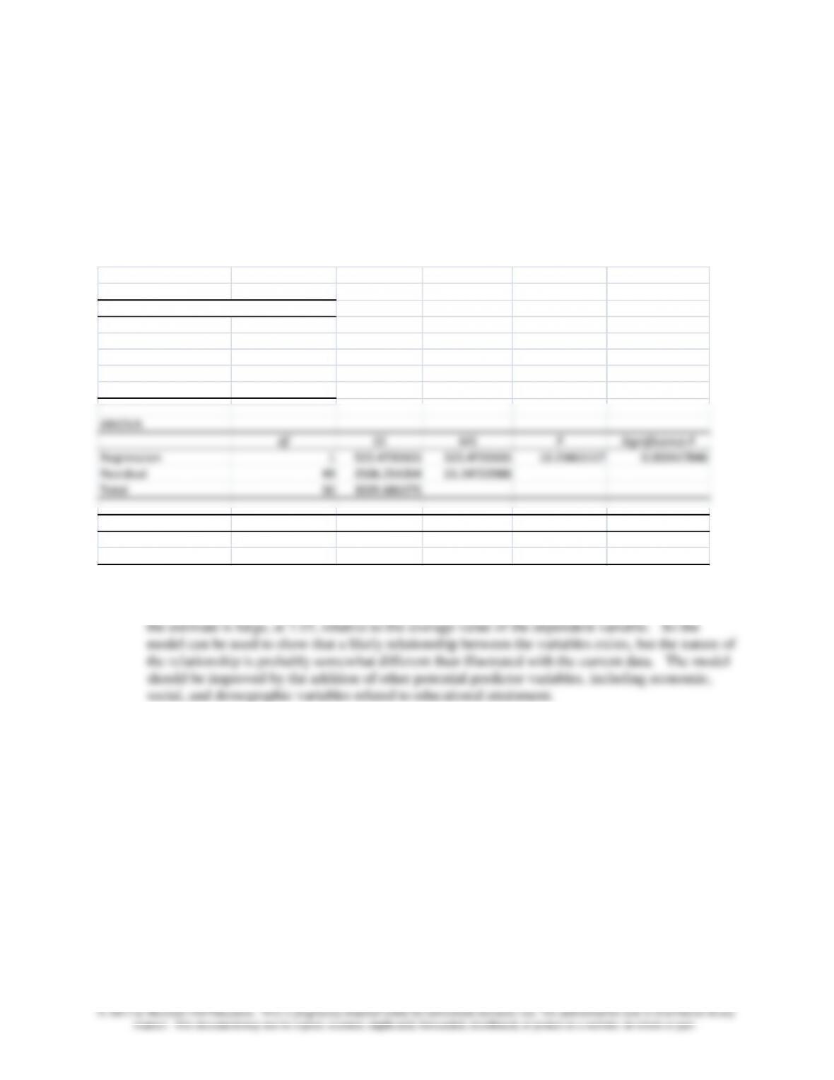
1. The regression results for the above data, shown in the Excel spreadsheet below, indicate that
there is a strong statistical relationship between percentage of children in poverty and graduation
rate; as expected the relationship is negative, that is, the higher the poverty rate, the lower the
graduation rate.
SUMMARY OUTPUT
Regression Statistics
Multiple R 0.415669255
R Square 0.172780929
Adjusted R Square 0.155898908
Standard Error 7.151729153
Observations 51
ANOVA
df SS MS F Significance F
Regression 1 523.4720103 523.4720103 10.23461117 0.002417846
Residual 49 2506.214264 51.14722988
Total 50 3029.686275
Coefficients Standard Error t Stat P-value Lower 95%
Intercept 85.37532874 3.073757551 27.77555722 1.20942E–31 79.1983818
Poverty -0.578221666 0.180741835 -3.199157884 0.002417846 -0.941435974
2. The t statistic for the poverty variable is strongly significant, but other measures are not good.
The R square of 17% is quite low, indicating a poorly fitting model. Also, the standard error of
Chapter 8 – Cost Estimation
Case 8-6: University Cost Forecasting
1. The following are four different regression models that were run on the Western
University data. See below for the regression results and an overall evaluation that
follows.
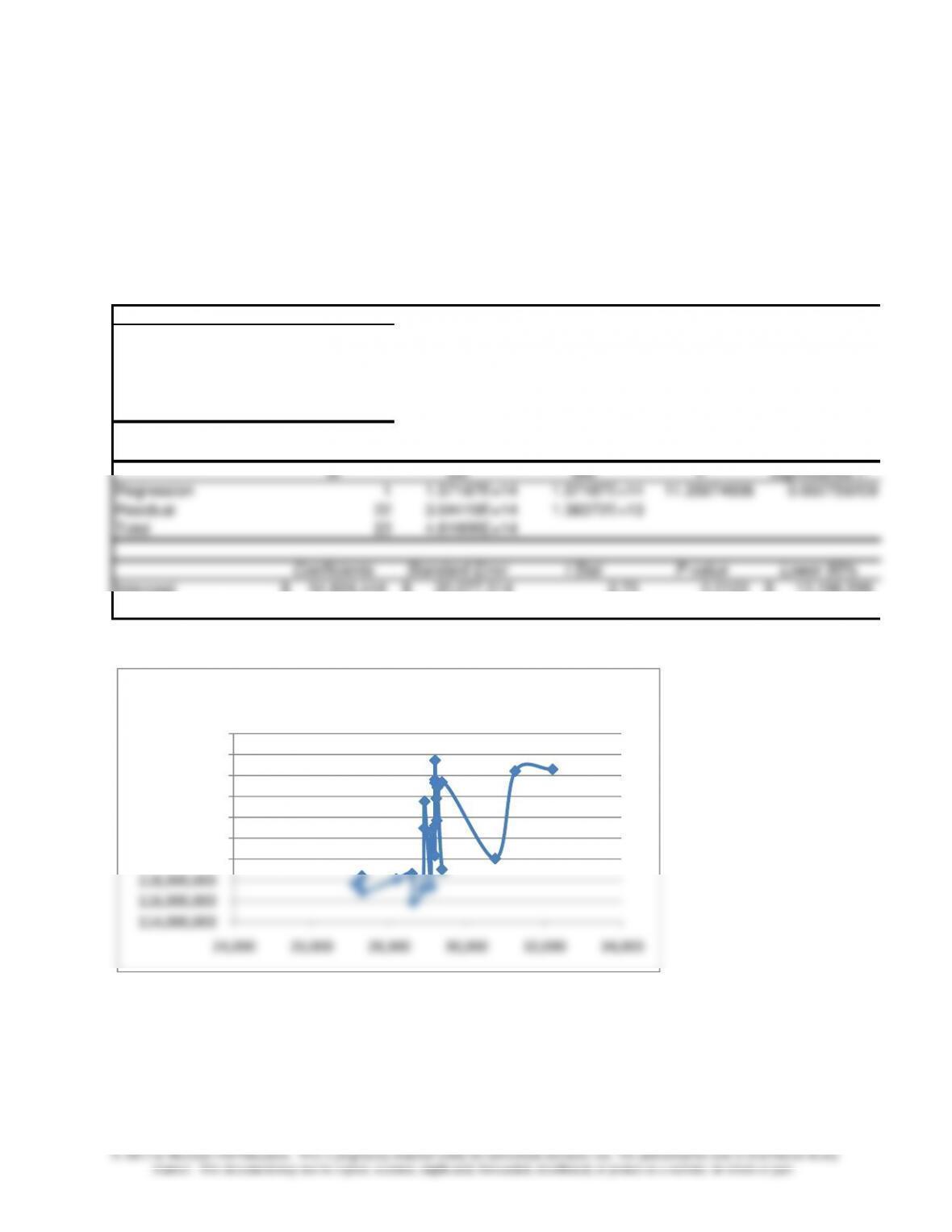
Regression One: Students Enrolled
Regression Statistics
Multiple R 0.5835
R Square 0.3405
Adjusted R Square 0.3105
Standard Error 3,719,841$
Observations 24
ANOVA
df SS MS F Significance F
Regression 1 1.57187E+14 1.57187E+14 11.35974606 0.002759209
Residual 22 3.04419E+14 1.38372E+13
Total 23 4.61606E+14
Coefficients Standard Error t Stat P-value Lower 95%
Intercept 54,824,444$ 20,077,314$ 2.73 0.0122 13,186,598$
Students enrolled 2,323$ 689$ 3.37 0.0028 893$
Plot of Regression One
114,000,000
116,000,000
118,000,000
120,000,000
122,000,000
124,000,000
126,000,000
128,000,000
130,000,000
132,000,000
24,000 26,000 28,000 30,000 32,000 34,000
Total Costs
Chapter 8 – Cost Estimation
8-15
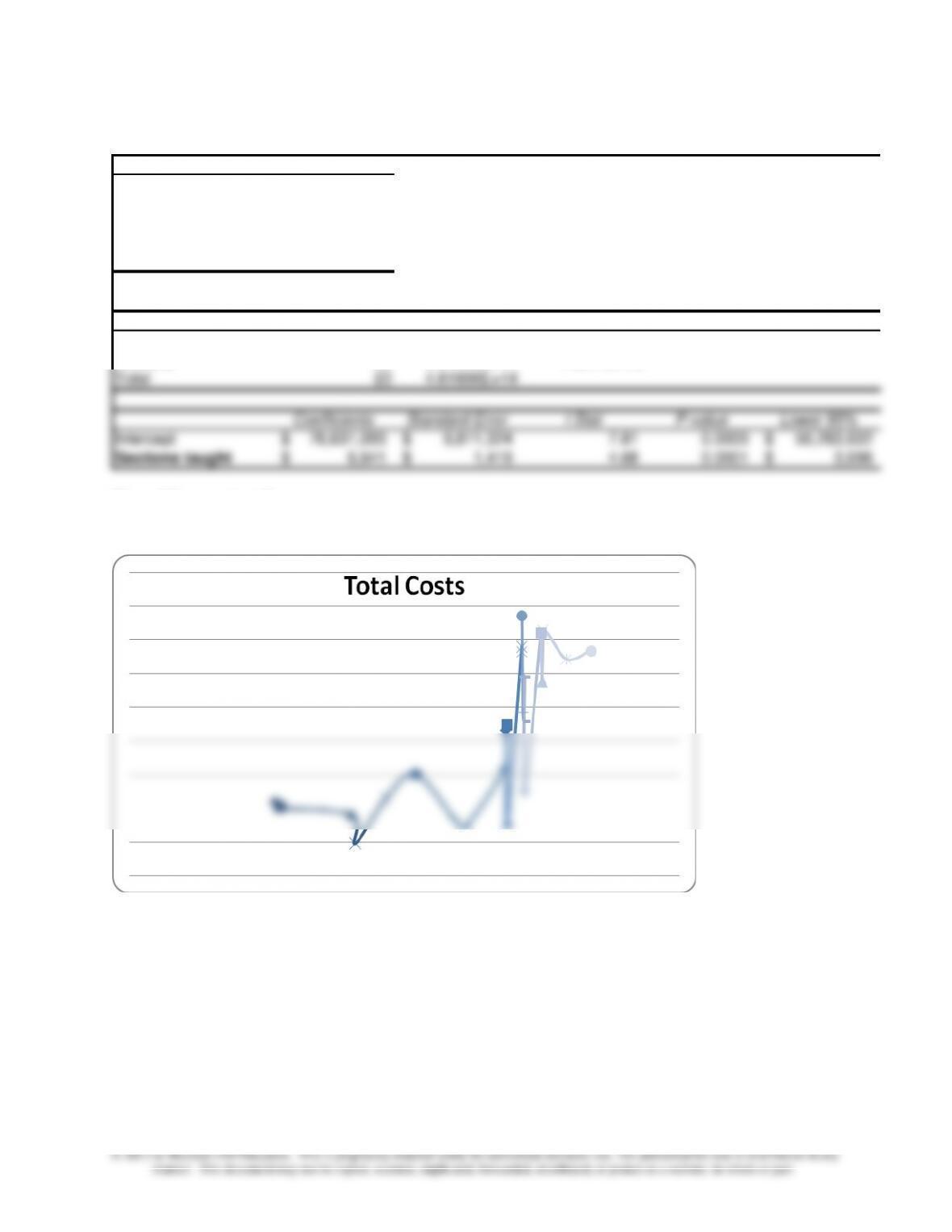
Regression Two: Sections Taught
Regression Statistics
Multiple R 0.7063
R Square 0.4989
Adjusted R Square 0.4761
Standard Error 3,242,531$
Observations 24
ANOVA
df SS MS F Significance F
Regression 1 2.30298E+14 2.30298E+14 21.90390541 0.000114606
Residual 22 2.31308E+14 1.0514E+13
Total 23 4.61606E+14
Coefficients Standard Error t Stat P-value Lower 95%
Intercept 76,631,093$ 9,811,324$ 7.81 0.0000 56,283,632$
Sections taught 6,641$ 1,419$ 4.68 0.0001 3,698$
Plot of Regression Two
Chapter 8 – Cost Estimation
8-16
Regression Three: Number of Courses Listed
Regression Statistics
Multiple R 0.5775
R Square 0.3335
Adjusted R Square 0.3032
Standard Error 3,739,627$
Observations 24
ANOVA
df SS MS F Significance F
Regression 1 1.5394E+14 1.5394E+14 11.00767923 0.00312726
Residual 22 3.07666E+14 1.39848E+13
Total 23 4.61606E+14
Coefficients Standard Error t Stat P-value Lower 95%
Intercept 55,592,702$ 20,164,166$ 2.76 0.0115 13,774,736$
Courses listed 24,040$ 7,246$ 3.32 0.0031 9,013$
Plot of Regression Three
Chapter 8 – Cost Estimation
8-17
Regression Four: Courses listed, Sections Taught, and Students Enrolled
Regression Statistics
Multiple R 0.8273
R Square 0.6845
Adjusted R Square 0.6371
Standard Error 2,698,662$
Observations 24
ANOVA
df SS MS F Significance F
Regression 3 3.15951E+14 1.05317E+14 14.46108252 3.05697E-05
Residual 20 1.45656E+14 7.28278E+12
Total 23 4.61606E+14
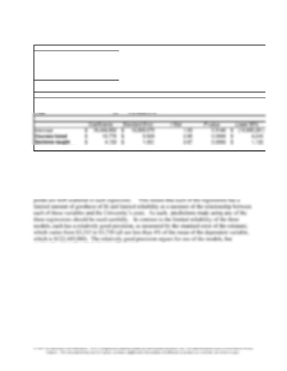
Coefficients Standard Error t Stat P-value Lower 95%
Intercept 19,464,902$ 18,869,075$ 1.03 0.3146 (19,895,281)$
Courses listed 15,778$ 5,529$ 2.85 0.0098 4,245$
Sections taught 4,159$ 1,451$ 2.87 0.0096 1,132$
Students enrolled 1,045$ 596$ 1.75 0.0948 (198)$
Overall Evaluation:
Each of the simple regressions on the three independent variables (regressions one, two,
and three) are significant at p < .01, and each have coefficients for the independent variable that
are in the expected direction and of a plausible amount. The adjusted R square for each
regression is low, however. Note from the plots for each regression shown above that the data
cautiously, given the relatively poor R square.
Chapter 8 – Cost Estimation
8-18
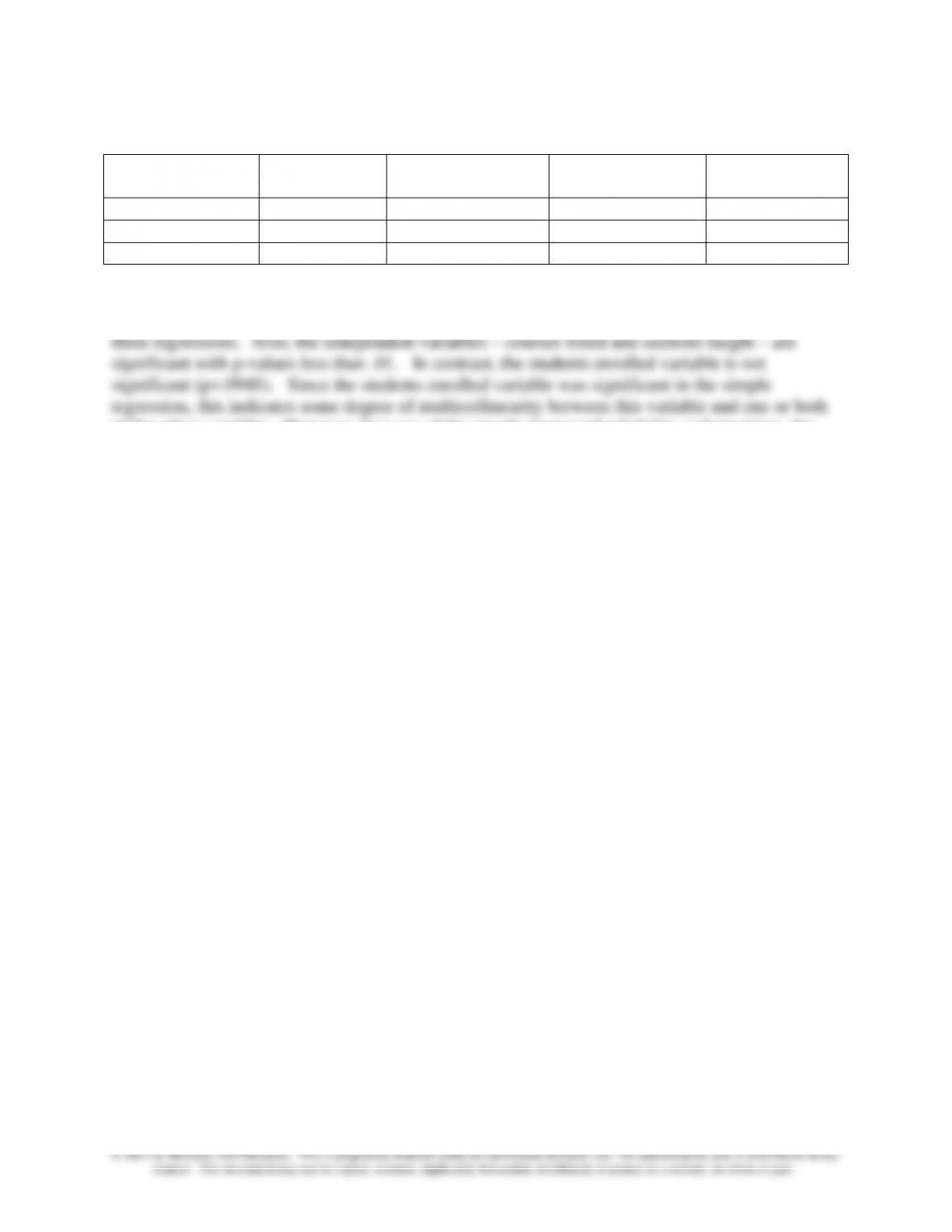
Adjusted R-
Square
Independent
Variable
Coefficient
P-value
Regression One
.3105
Students enrolled
$2,323
.0028
Regression Two
.4761
Sections taught
$6,641
.0001
Regression Three
.3032
Courses listed
$24,040
.0031
The multiple regression, regression four, includes all three independent variables and has
higher R square (.6371), and lower standard error of the estimate ($2,698) than any of the prior
of the other variables. However, because of the greatly improved reliability and precision, the
multiple regression model is the best choice for predicting University costs.
2. The above analysis can be compared to activity-based costing because it takes a multiple
cost driver approach to forecasting total cost.
Chapter 8 – Cost Estimation
8-19
Teaching Strategy for Reading
“How to Find the Right Bases and Rates”
This article shows an actual application of regression analysis for determining multiple overhead
rates using the spreadsheet software. The article explains the interpretation of the R-squared and t-values
and provides a good discussion of when regression analysis is useful.
Discussion Questions:
1. What is regression analysis used to accomplish in this article?
The regression analysis is used to determine the best cost drivers to use when using multiple overhead
2. What are the steps to perform a simple regression analysis?
The use of regression, as explained in this article, requires a spreadsheet program such as EXCEL, and the
3. What does Table 4 tell you? Which cost driver would you pick for each cost type⎯maintenance,
packaging, materials handling, storage, and production scheduling?
Table 4 provides the information we need to determine which single cost driver provides the best
fit for each cost type:
• maintenance: machine hours
• packaging: pounds of material
additional statistical reliability.