Chapter 16 – Operational Performance Measurement: Further Analysis of Productivity and Sales
16–31
16–46 Direct Labor Variances, Productivity Measures, and Standard
Costs (30 min)
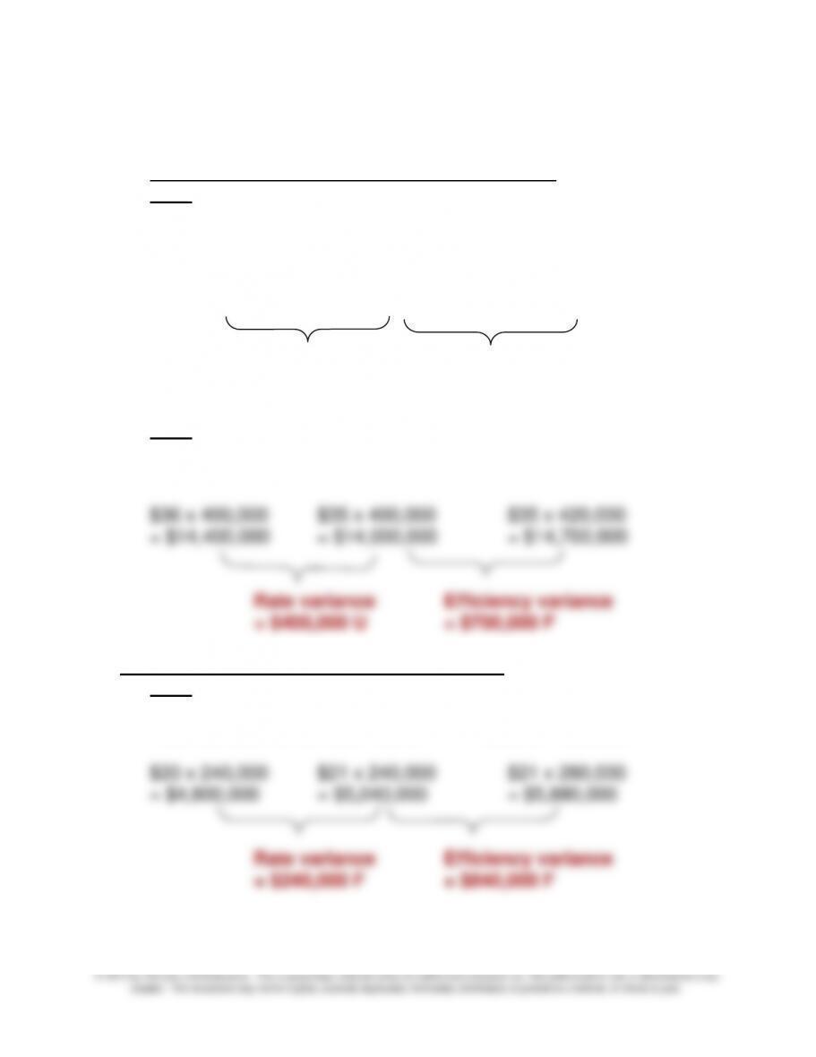
1. Assembly Department Direct Labor Variances
2012:
Total actual direct labor hours: 25 x 20,000 = 500,000
Total standard direct labor hours: 24 x 20,000 = 480,000
$30 x 500,000 $28 x 500,000 $28 x 480,000
= $15,000,000 = $14,000,000 = $13,440,000
Rate variance Efficiency variance
= $1,000,000 U = $560,000 U
2013:
Total actual direct labor hours: 20 x 20,000 = 400,000
Total standard direct labor hours: 21 x 20,000 = 420,000
Testing Department Direct Labor Variances
2012:
Total actual direct labor hours: 12 x 20,000 = 240,000
Total standard direct labor hours: 14 x 20,000 = 280,000
16–32
16-46 (continued –1)
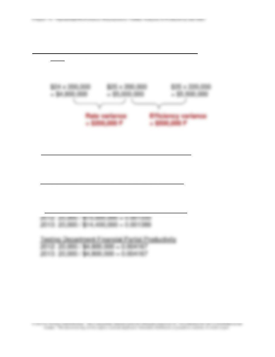
Testing Department Direct Labor Variances (continued)
2013:
Total actual direct labor hours: 10 x 20,000 = 200,000
Total standard direct labor hours: 11 x 20,000 = 220,000
2. Assembly Department Operational Partial Productivity
2012: 20,000 / 500,000 = 0.04
2013: 20,000 / 400,000 = 0.05
Testing Department Operational Partial Productivity
2012: 20,000 / 240,000 = 0.083333
2013: 20,000 / 200,000 = 0.1
3. Assembly Department Financial Partial Productivity
Chapter 16 – Operational Performance Measurement: Further Analysis of Productivity and Sales
16–33
16-46 (continued –2)
4. Recap:
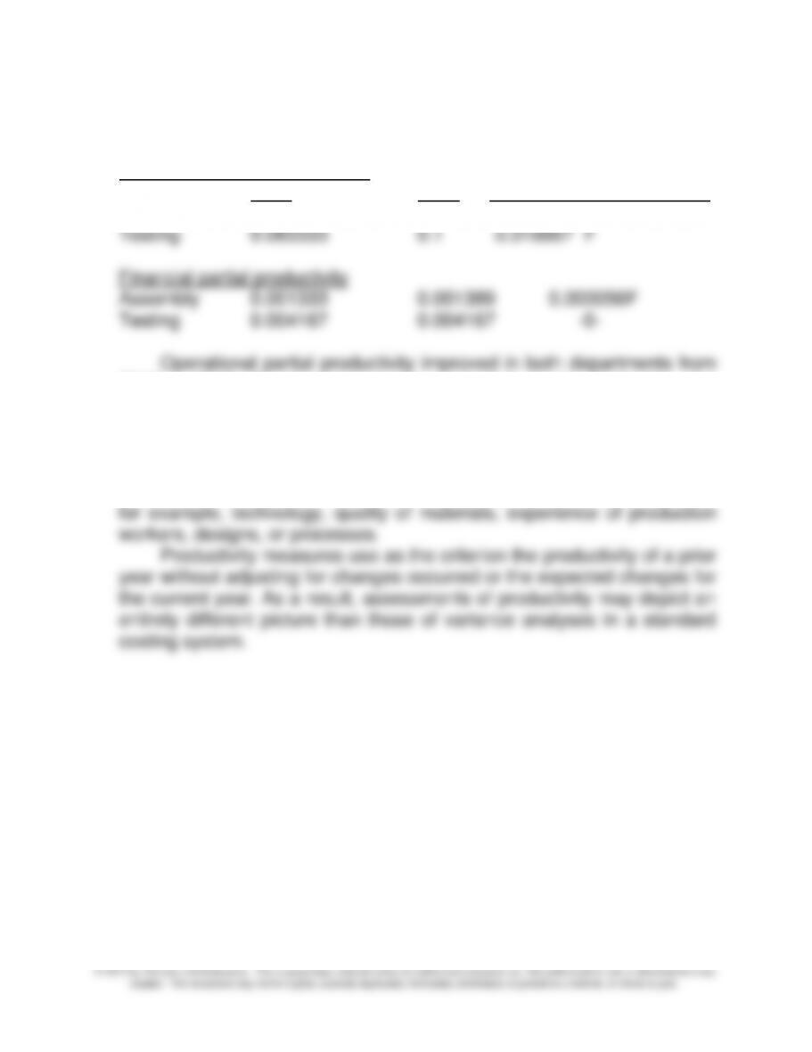
Operational partial productivity
2012 2013 Change
Assembly 0.04 0.05 0.01 F
2012 to 2013. The financial partial productivity in the Assembly also
improved while the Testing remained unchanged.
5. The standards in a standard costing system often are determined
independently and incorporate changes in operating factors. The
standard for the operation of a year may change because of changes in,
Chapter 16 – Operational Performance Measurement: Further Analysis of Productivity and Sales
16–34
16-47 Productivity and Market Share in the Auto Industry; Internet
Exercise (20 min)
1.
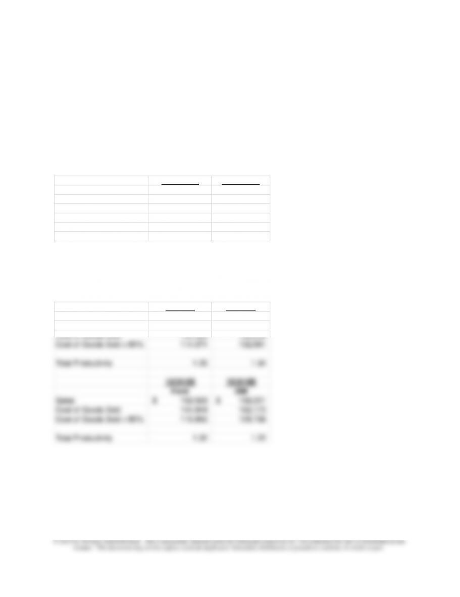
The total productivity for the auto makers is shown below for 2010, the
most recent year at the time the question was prepared in October 2011.
Also, while not required, the results for 2007 and 2005 are also shown for
comparison.
12/31/2010 12/31/2010
Ford GM
Sales 128,954$ 135,592$
Cost of Goods Sold 122,296 130,508
Cost of Goods Sold x 80% 97,837 104,406
Total Productivity 1.32 1.30
For contrast, the productivity calculations for the two companies in 2007
and 2005 are as follows:
12/31/07 12/31/07
Ford GM
Sales 154,379$ 178,199$
Cost of Goods Sold 142,589 166,239
Cost of Goods Sold x 80% 114,071 132,991
Total Productivity 1.35 1.34
12/31/05 12/31/05
Ford GM
Sales 153,503$ 158,221$
Cost of Goods Sold 144,944 162,173
Cost of Goods Sold x 80% 115,955 129,738
Total Productivity 1.32 1.22
The objective of this question is to make the students aware that total
productivity can be at least approximated for a company the student is
interested in by obtaining basic financial data from the firm’s annual report.
Chapter 16 – Operational Performance Measurement: Further Analysis of Productivity and Sales
16–35
16-47 (continued –1)
Note there are no significant differences between the auto makers or
between the productivity measures for 2005, 2007, and 2010. Note that this
is in contrast to the Harbour Report data on auto firm productivity in 2008,
cited in Problem 16-35, which reports an increase in productivity
(measured as labor hours per vehicle) for Ford. The two measures of
productivity do not measure the same thing, so that these differences arise.
While the measures computed here are limited by the amount of
information available, they can provide a starting point for looking at other
measures of performance, and looking for more detailed information about
From Ford’s 2010 Annual Report:
“…Total costs and expenses for our Automotive sector for 2010 and 2009
was $113.5 billion and $107.2 billion,respectively, a difference of $6.3
billion. An explanation of the change is shown below (in billions):
2010(Over)/Under2009
Explanation of Change:
Volume and Mix, and Exchange (11.6)
Material Costs Excluding Commodity Costs 1.1
Chapter 16 – Operational Performance Measurement: Further Analysis of Productivity and Sales
16–36
16-47 (continued -2)
Ford’s 2005 Annual Report has a similar analysis
Increase (decrease)
Supplier related cost $1
Pension and health care .8
Warranty costs .4
Depreciation and amortization (investments
2. This requirement can be assigned for class discussion, and answers will
likely vary, depending on what portion of the financial statement is used
and which year’s annual report is used. The discussion here can focus on
some of the following (all these points are based on the 2010, 2007 and
2005 annual reports of GM and Ford)
Alternatively, the instructor can assign requirement 1 only, and then
discuss some of the observations about requirement 2, as noted below.
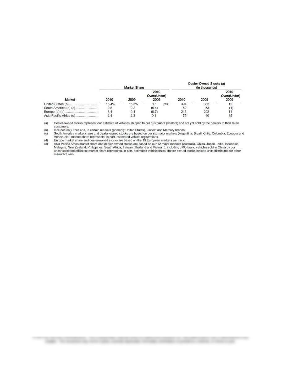
• some firms will be improving market share in some markets and
losing in others; for example Ford lost market share in the Europe
Chapter 16 – Operational Performance Measurement: Further Analysis of Productivity and Sales
16–37
16-47 (continued -3)
Chapter 16 – Operational Performance Measurement: Further Analysis of Productivity and Sales
16–38
16–48 Productivity and Ethics (15 min)
1. The operational partial productivity deteriorates slightly from
0.0051 in 2012 (500/99,000) to 0.005 in 2013 (560/112,000).
2. Kim Tomas should not follow the order without following a
consistent accounting method. If the firm believes that certain
Chapter 16 – Operational Performance Measurement: Further Analysis of Productivity and Sales
16–39
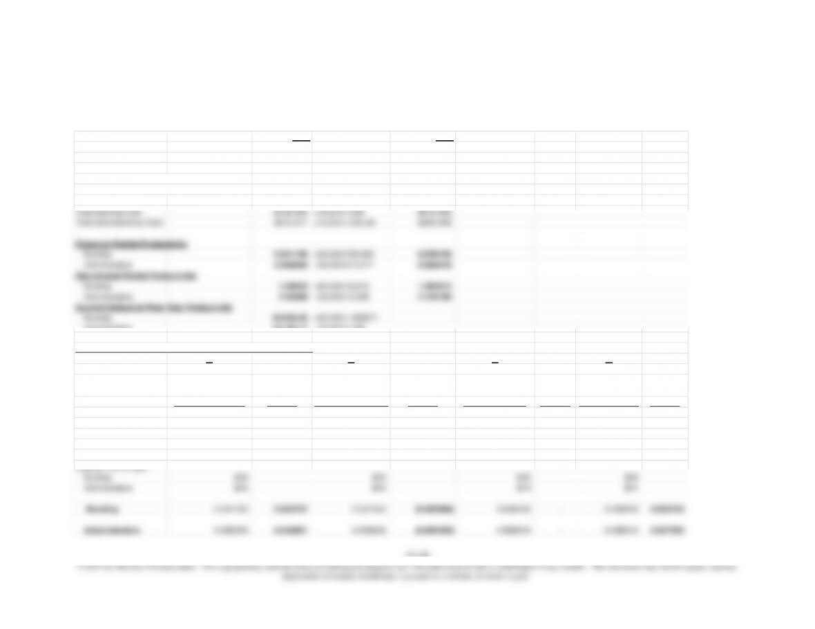
16–49 Partial Operational and Financial Productivity; Medical Practice (45 min)
1.,2. Partial operational and financial productivity and separation of partial financial productivity:
2013 2012
Patient visits 30,000 26,000
Nursing hours used 18,675 17,800
Administrative hours used 12,225 12,225
Cost of nursing support per hour $39.00 $38.00
Cost of administrative suppor per hour $25.56 $24.00
Total Nursing Cost $728,325 =18,675 x $39 $676,400
Total Administrative Cost $312,471 =12,225 x $25.56 $293,400
Financial Partial Productivity
Nursing 0.041190 =30,000/728,325 0.038439
Administrative 0.096009 =30,000/312,471 0.088616
Operational Partial Productivity
Nursing 1.60643 =30,000/18,675 1.460674
Administrative 2.45399 =30,000/12,225 2.126789
Output 30,000 30,000 30,000 26,000
Input Amount
Nursing 18,675 20,538 20,538 17,800
Administrative 12,225 14,106 14,106 12,225
Cost per unit of input
Nursing $39 $39 $38 $38
Administrative $26 $26 $24 $24
Nursing 0.041190 0.003737 0.037453 (0.000986) 0.038439 – 0.038439 0.002752
Administrative 0.096009 0.012801 0.083208 (0.005409) 0.088616 – 0.088616 0.007393
Chapter 16 – Operational Performance Measurement: Further Analysis of Productivity and Sales
16–40
16–49 (continued –1)
3.
MEMO
TO: Rajat Patel, Integrated Medical Care
FROM: Joseph Marin, Marin & Associates
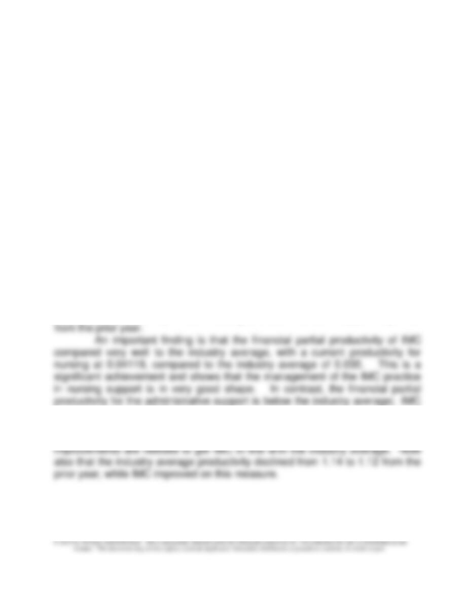
I have calculated the financial partial productivity measure for IMC for
the current and prior year and the supporting documentation is attached.
Nursing productivity improved by 0.003737 over the prior year, while
administrative productivity improved by 0.012801. I attribute this to the
greater than 15% increase in patient demand, with only modest increases in
nursing hours, and no increase in administrative hours. These figures show
that the practice is managed very effectively.
There was a small decline in the pricing component of productivity,
since average wages increased in both nursing and administrative support;
overall, taking both the change in wages and change in hours into account,
the financial productivity of both nursing and administrative support improved
has productivity of 0.096 in the current year relative to the industry average of
1.12. The good news, as noted above, is that the productivity of the
administrative support area is improving relative to the prior year, and these
Chapter 16 – Operational Performance Measurement: Further Analysis of Productivity and Sales
16–41
16-49 (continued –2)
Medical practices are under pressure in recent years as Medicare
reimbursements have fallen and technology and labor costs have
increased. Many practices have looked for increased productivity and
profitability through:
1. Cross-training employees so that overall staff positions can be
reduced as employee are able to perform a variety of tasks
trend is for the single-doctor practice to be declining in numbers, as
more and more medical practices consolidate.
Source: Katherine Reynolds Lewis, “Medical Practices Work on Ways to
Serve Patients and Bottom Line,” The New York Times, September 8,
2011, p. B10.

4.
16–50 Flexible Budget, Sales Volume, Sales Mix, and Sales Quantity
Variances (40 min)
1.
Total per unit or % Total per unit or %
Sales
Product A 180,400$ 110.00$ 240,000$ 120.00$
Product B 341,120 52.00 300,000 50.00
Total 521,520$ 540,000$
Sales Units
Product A 1,640$ 20.00% 2,000$ 25.00%
Product B 6,560 80.00% 6,000 75.00%
Total 8,200$ 8,000$
Variable Cost
Product A 106,600$ 65.00$ 140,000$ 70.00$
Product B 216,480 33.00 180,000 30.00
Total 323,080$ 320,000$
Contribution Margin
Product A 73,800$ 45$ 100,000$ 50.00$
Product B 124,640 19.00 120,000 20.00
Total 198,440$ 220,000$
Fixed cost
Product A 80,000$ 80,000$
Product B 40,000 40,000
Total 120,000$ 120,000$
Contribution Income Statement
Sales Price Flexible Sales Volume
Sales
Actual Variance Budget Variance Budget
Product A 180,400$ (16,400) $196,800 (43,200) 240,000$
Product B 341,120
13,120 328,000 28,000
300,000
Operating Income 78,440$ 100,000$
ABC=A+B
Sales Mix Sales Quantity Volume
Variance Variance Variance
Product A
(20,500)$ =(.20-.25)x8200x50 2,500$ =(8200-8000)x.25×50 (18,000)$
Product B
8,200$ =(.80-.75)x8200x20 3,000$ =(8200-8000)x.75×20 11,200
(12,300)$ 5,500$ (6,800)$
Actual
Budget
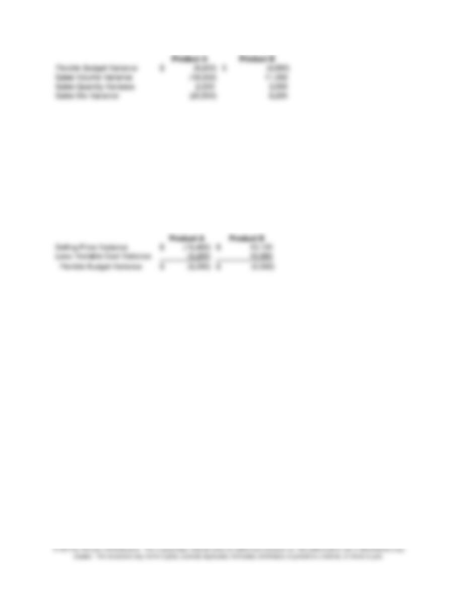
Summary of Variances, as calculated above in contribution margin
Chapter 16 – Operational Performance Measurement: Further Analysis of Productivity and Sales
16–43
Product A Product B
Flexible Budget Variance (8,200)$ (6,560)$
Sales Volume Variance (18,000) 11,200
Sales Quantity Variance 2,500 3,000
Sales Mix Variance (20,500) 8,200
16-50 (continued –1)
2.
The reconciliation of the selling price, variable cost, and flexible cost
variances is as follows. The variances are in the solution shown in part 1.
A negative selling price variance means an unfavorable variance and a
positive is favorable. A negative variable cost variance means a favorable
variance and a positive is unfavorable.
Product A Product B
Selling Price Variance (16,400)$ 13,120$
Less: Variable Cost Variance (8,200) 19,680
Flexible Budget Variance (8,200)$ (6,560)$
Chapter 16 – Operational Performance Measurement: Further Analysis of Productivity and Sales
16–51 Flexible Budget, Sales Volume, Sales Mix, and Sales Quantity
Variances (30 min)
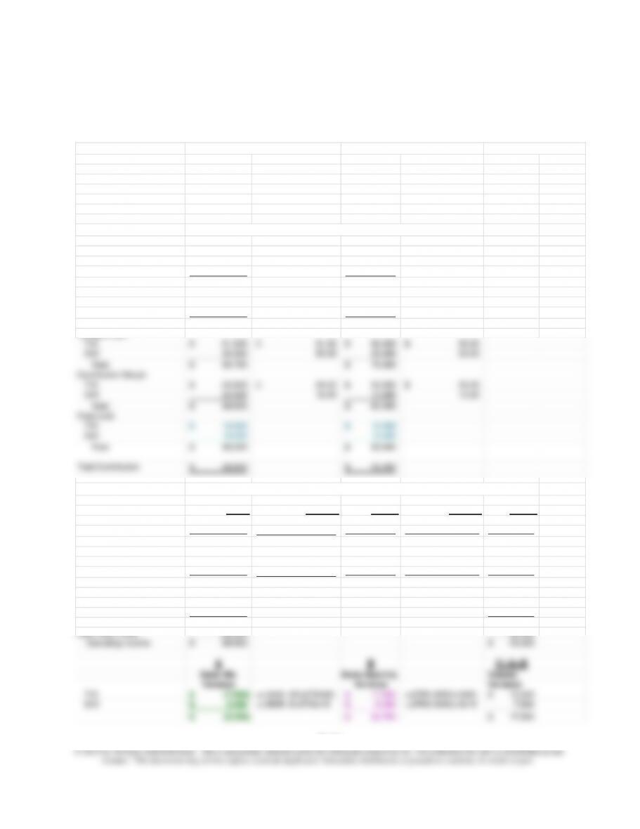
1.
T10 S40 T10 S40 Actual Budget
Units sold 1,200 1,500 1,000 1,000 2,700 2,000
Sales Dollars 126,000$ 58,500$ 100,000$ 40,000$ 184,500$ 140,000$
Sales Price 105.00$ 39.00$ 100.00$ 40.00$
Variable Cost 61,200$ 34,500$ 50,000$ 25,000$ 95,700$ 75,000$
Unit Variable Cost 51.00$ 23.00$ 50.00$ 25.00$
Total per unit or % Total per unit or %
Sales
T10 126,000$ 105.00$ 100,000$ 100.00$
S40 58,500 39.00 40,000 40.00
Total 184,500$ 140,000$
Sales Units
T10 1,200 44.44% 1,000 50.00%
S40 1,500 55.56% 1,000 50.00%
Total 2,700 2,000
Variable Cost
T10 61,200$ 51.00$ 50,000$ 50.00$
S40 34,500 23.00 25,000 25.00
Total 95,700$ 75,000$
Contribution Margin
T10 64,800$ 54.00$ 50,000$ 50.00$
S40 24,000 16.00 15,000 15.00
Total 88,800$ 65,000$
Fixed cost
T10 10,000$ 10,000$
S40 10,000 10,000
Total Variable Costs 95,700$ (1,800)$ 97,500$ 22,500$ 75,000$
Contribution
T10 64,800$ 4,800$ 60,000$ 10,000$ 50,000$
S40 24,000
1,500 22,500 7,500 15,000
Total Contribution 88,800$ 65,000$
Less Fixed Costs 20,000
20,000
Operating Income 68,800$ 45,000$
A B C=A+B
Sales Mix Sales Quantity Volume
Variance Variance Variance
T10 (7,500)$ =(.4444-.50)x2700x50 17,500$ =(2700-2000)x.5x50 10,000$
S40 2,250$ =(.5555-.5)x2700x15 5,250$ =(2700-2000)x.5x15 7,500
(5,250)$ 22,750$ 17,500$
Actual
Budget
Contribution Income Statement
Total
Chapter 16 – Operational Performance Measurement: Further Analysis of Productivity and Sales
16–45
16–51 (continued -1)
The solution is summarized below, and the calculations are shown above
(a negative is unfavorable and a positive is favorable):
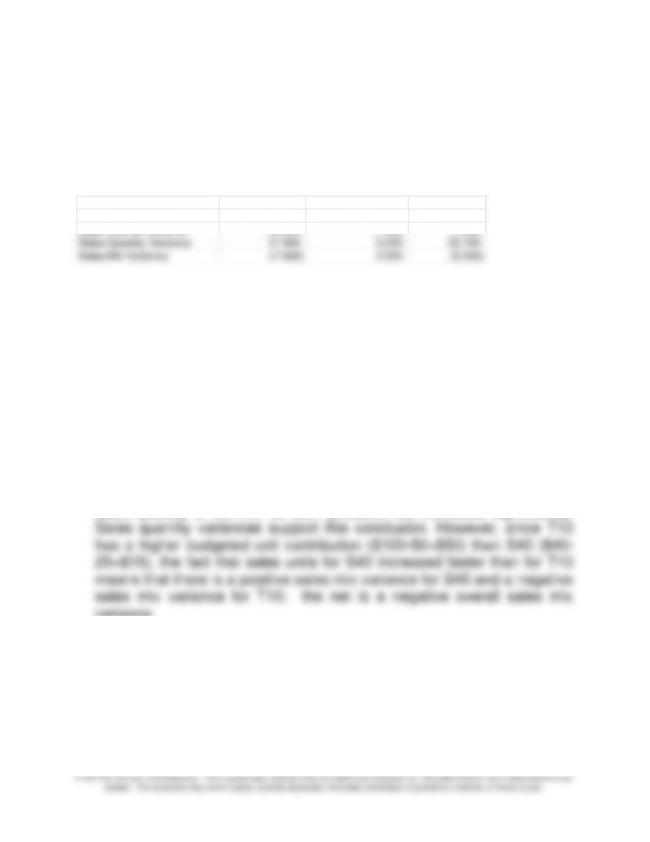
T10 S40 Total
Flexible Budget Variance 4,800$ 1,500$ 6,300$
Sales Volume Variance 10,000 7,500 17,500
Sales Quantity Variance 17,500 5,250 22,750
Sales Mix Variance (7,500) 2,250 (5,250)
2.
MEMO
TO: Jay Banning, CEO
FROM: I M Student
RE: Banning Inc. Variance Analysis
The following information describes the results of variances
calculated on the attached spreadsheet (see requirement 1) with regard
to what was planned for 2013 and the actual results reported.
The firm has a favorable sales volume variance for both T10 and S40
due to increase sales volumes over budget for both products. The total
sales quantity of the firm for both products has increased significantly.
variance.
The flexible budget variance is favorable for both S40 and T10
because T10’s increase in price was greater than its small increase in
unit variable cost; for S40, the small decrease in price was more than
recovered by the substantial decrease in unit cost for S40.
Please contact me for further discussion.