
Chapter 16 – Operational Performance Measurement: Further Analysis of Productivity and Sales
16–16
16-36 Productivity and the Economy (20 min)
This question is intended for class discussion. Answers are likely to vary.
Here are some points that could be brought up in the discussion.
It is clear from the BLS predictions and preliminary quarterly measures for
2009 that the rate of productivity increase has fallen from the levels of the
prior few years. Some would argue that the very high rates in 2002 and
2003 were the result of significant workforce reductions by firms in reaction
to the market downturn of 2000-2001. The laid-off workers were rehired
only after businesses were comfortable about the growth in the economy.
Some economists view this as a natural part of the business cycle.
The decline in investment in both capital expenditures and information
technology in 2009 suggests that productivity growth will be reduced
somewhat in the coming few years. However, others note that investment
in information technology can take several years to affect productivity, so
that the recent investments may carry forward for several years beyond
2009.
As in the period of 2000-2001, significant employment reductions have had
the effect of boosting productivity. Note the increase in 2009. The
increase in productivity continued into 2010 with an annual productivity of
4.1, the highest since 2002. However, the first half of 2011 showed a
decline in productivity, to -.0.6. The reasons cited were the increase in
wages and slower pace of workforce reductions during this period. Note
how the pattern of increase in productivity in periods of workforce reduction
(2001-2003, and 2008-2010) are followed by periods of lower productivity.
The reason is that the large workforce reductions show significant gains in
productivity which are difficult to maintain without further layoffs which are
not indicated by the strengthening economy in 2010-11.
Most economists accurately predicted that productivity would increase in
2009 – 2010, but these economists are advising that the next few years will
show lower, perhaps much lower productivity. The figures for 2011 and the
first quarter of 2012 are consistent with that (most recent data as of June
2012).

16–17
© 2013 by McGraw-Hill Education. This is proprietary material solely for authorized instructor use. Not authorized for sale or distribution in any
manner. This document may not be copied, scanned, duplicated, forwarded, distributed, or posted on a website, in whole or part.
16-36 (continued –1)
U.S. Census Bureau (capital investment data; most recent data in October
2011 was for the year 2009):
http://www.census.gov/compendia/statab/cats/business_enterprise/investm
ent_capital_expenditures.html
Bureau of Labor Statistics (nonfarm business productivity):
http://data.bls.gov/timeseries/PRS85006092
Useful additional sources: “America’s Productivity Growth Has Slowed;
Does that Matter?” The Economist, April 16, 2007; “Not Dead, Just
Resting,” The Economist, October 11, 2008, p. 18; Productivity Falls for
Second Quarter in a Row,” The Wall Street Journal, August 10, 2011, p.
B9; “A Jump in Labor Costs,” Bloomberg Businessweek, August 29, 2011,
p. 16.
Chapter 16 – Operational Performance Measurement: Further Analysis of Productivity and Sales
16–18
16-37 Alternative Measures of Productivity (20 min)
The measure based on manufacturing capacity utilization has a meaningful
interpretation in the sense that it captures the rate of utilization of invested
dollars. It ties in very well with the concept of return on assets (net income
over total assets), a key measure of business performance that is covered
in chapter 19. Managers and investors would like to see high return on
measures are more controllable by managers since some portion of
manufacturing costs can be controlled in the short term. As such, it is a
more useful measure of operational level performance. The measure of
capacity level utilization is a productivity measure with a longer term focus,
and is more appropriate for management level control.
For capacity utilization data, see:
http://www.federalreserve.gov/releases/g17/current/
Chapter 16 – Operational Performance Measurement: Further Analysis of Productivity and Sales
16–19
16–38 Productivity Measures for Call Centers (20 min)
The measure proposed, number of calls/number of hours, is a common
and intuitive measure of productivity. The management of the call center
could track this productivity over time to (1) assess the productivity of the
call center staff (how long it takes to respond to a call) and (2) the overall
capacity in the call center (are we overstaffed?). A problem with the
measure is that one goal of the call center is to produce satisfied customers
Chapter 16 – Operational Performance Measurement: Further Analysis of Productivity and Sales
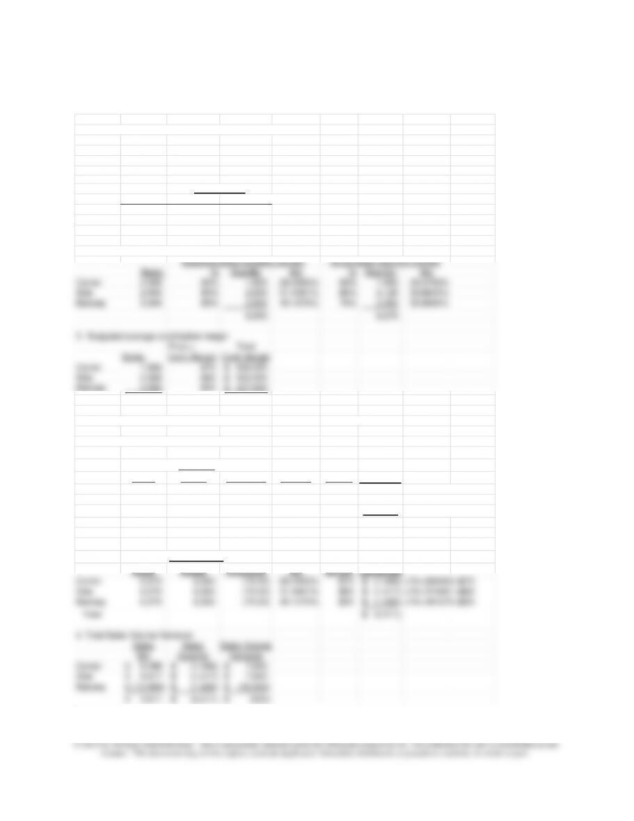
16–39 Sales Volume, Sales Quantity, and Sales Mix Variances (30 min)
DATA
Center 2,000
Side 2,500
Balcony 3,000
Ticket
Price Budget Actual Seats
Center $70 90% 95%
Side 60 80% 85%
Balcony 50 85% 75%
1. Budgeted and Actual Sales Mix Percentages
Seats % Quantity Mix % Quantity Mix
Center 2,000 90% 1,800 28.3465% 95% 1,900 30.2789%
Side 2,500 80% 2,000 31.4961% 85% 2,125 33.8645%
Balcony 3,000 85% 2,550 40.1575% 75% 2,250 35.8566%
6,350 6,275
2. Budgeted average contribution margin
Price = Total
Seats Cont. Margin Cont. Margin
Center 1,800 $70 126,000$
Balcony 35.8566% 40.1575% (0.043009) 6,275 $50 (13,494)$ =0.043009 x6,275x$50
Total 3,911$
Budgeted Budgeted Sales
Sales CM Quantity
Actual Budget Difference Mix per unit Variance
Center 6,275 6,350 (75.00) 28.3465% $70 (1,488)$ =75x.283465 x$70
Side 6,275 6,350 (75.00) 31.4961% $60 (1,417)$ =75x.314961 x$60
Balcony 6,275 6,350 (75.00) 40.1575% $50 (1,506)$ =75x.401575 x$50
Total (4,411)$
4. Total Sales Volume Variance
Sales Sales
Sales Volume
Mix Quantity Variance
Center 8,488$ (1,488)$ 7,000$
Side 8,917$ (1,417)$ 7,500$
Balcony (13,494)$ (1,506)$ (15,000)$
Sales Quantity
Number of seats available:
Percentages
Budgeted Sales Quantity and Mix
Actual Sales Quantity and Mix
16–21
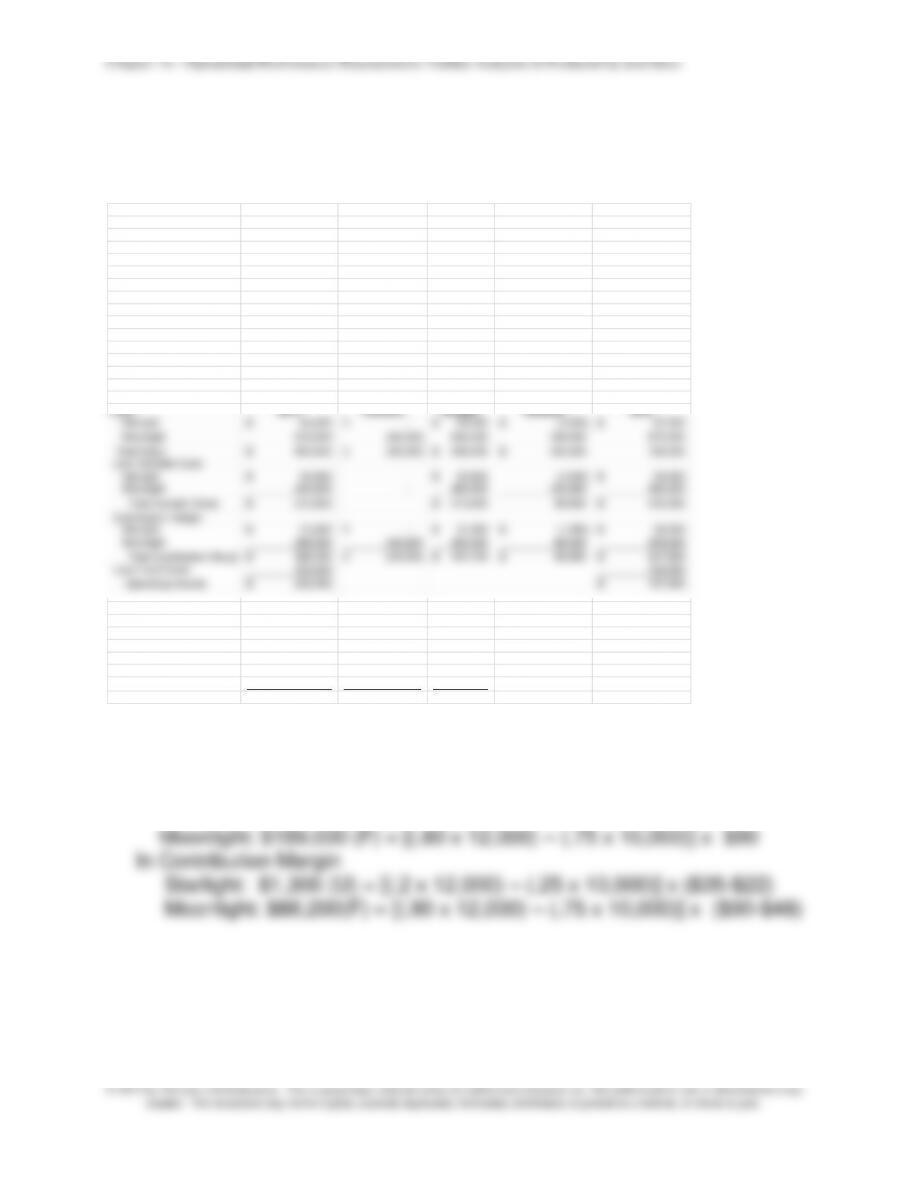
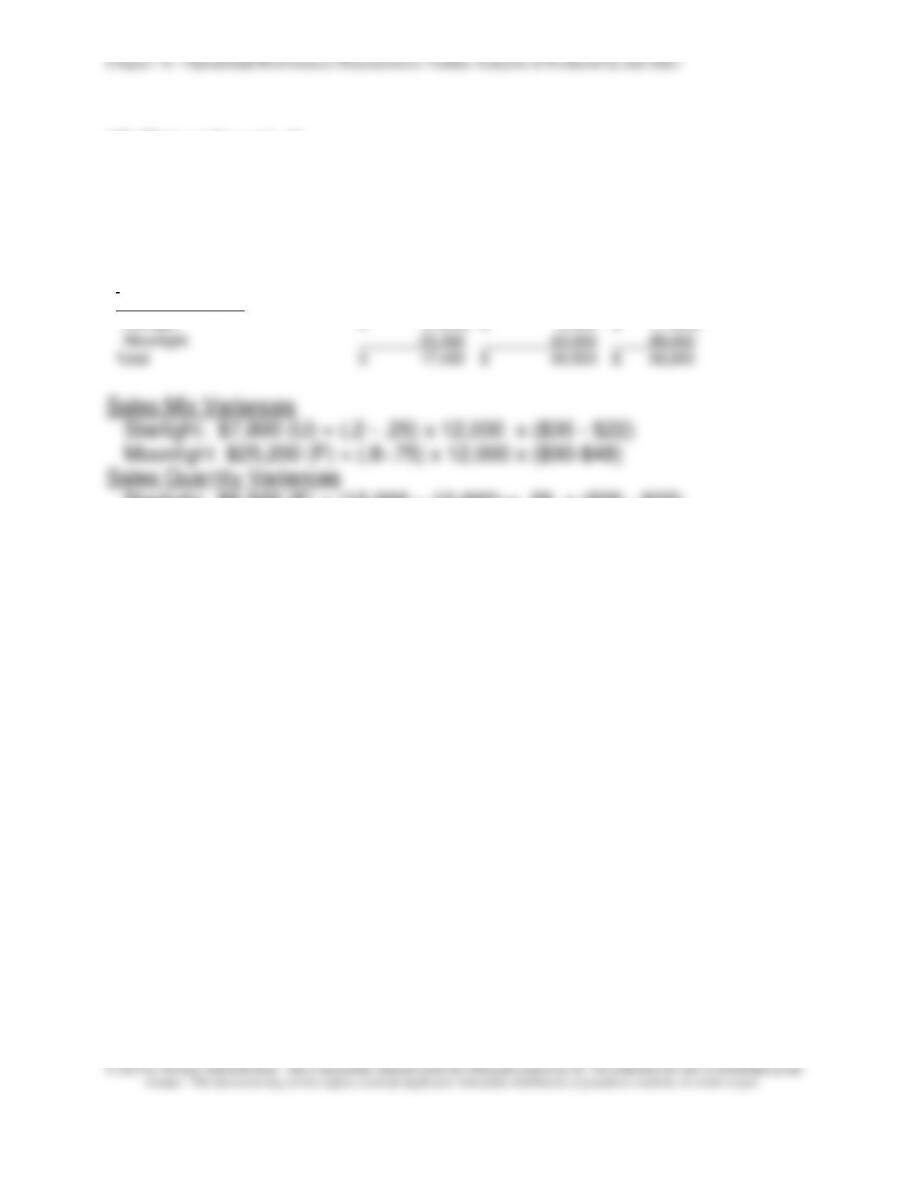
16-40 Sales Mix and Quantity Variances (20 min)
1. Contribution Income Statement for Hathaway
2013 2012
Sales Units 12,000 10,000
Sales Mix for each Product
Starlight 20% 25%
Moonlight 80% 75%
Price
Starlight 35.00$ 35.00$
Moonlight 85.00$ 90.00$
Variable Cost per Unit
Starlight 22.00$ 22.00$
Moonlight 48.00$ 48.00$
Fixed cost 150,000$ 150,000$
Sales Price Flexible Sales Volume
Sales 2013 Variance Budget Variance 2012
Starlight 84,000$ –$ 84,000$ (3,500)$ 87,500$
Moonlight 816,000 (48,000) 864,000 189,000 675,000
Total Sales 900,000$ (48,000)$ 948,000$ 185,500$ 762,500
Less Variable Costs
Starlight 52,800$ – 52,800$ (2,200) 55,000$
Moonlight 460,800 – 460,800 100,800 360,000
Total Variable Costs 513,600$ 513,600$ 98,600 415,000$
Contribution Margin
Starlight 31,200$ –$ 31,200$ (1,300)$ 32,500$
Moonlight 355,200 (48,000) 403,200 88,200 315,000
Total Contribution Margin
386,400$ (48,000)$ 434,400$ 86,900$ 347,500$
Less Fixed Costs 150,000 150,000
Operating Income 236,400$ 197,500$
Sales Mix Sales Quantity Volume
Variance Variance Variance
Starlight (7,800)$ 6,500$ (1,300)$
Moonlight 25,200 63,000 88,200
17,400$ 69,500$ 86,900$
2. The volume variances for each product are shown above:
In Sales Dollars:
Starlight: $3,500 (U) = [(.2 x 12,000) – (.25 x 10,000)] x $35
16–22
16-40 (continued –1)
3. The mix and quantity variances for each product are shown below;
note that the total of the sales mix and quantity variance equals the volume
variance
Starlight: $6,500 (F) = (12,000 – 10,000) x .25 x ($35 – $22)
Moonlight $63,000 (F) = (12,000 – 10,000) x .75 x ($90-$48)
Sales Mix Sales Quantity Volume
Contribution Margin
Variance Variance Variance
Starlight (7,800)$ 6,500$ (1,300)$
Moonlight 25,200
63,000
88,200
Total 17,400$ 69,500$ 86,900$
Chapter 16 – Operational Performance Measurement: Further Analysis of Productivity and Sales
16–23
PROBLEMS
16-41 Operational Partial Productivity (15 min)
1. Operational Partial Productivity
2013 2012
2. Productivity of direct material, CT140, deteriorated from 0.9697 in
2012 to 0.75 in 2013. Productivity of direct labor, however, remained
16–24
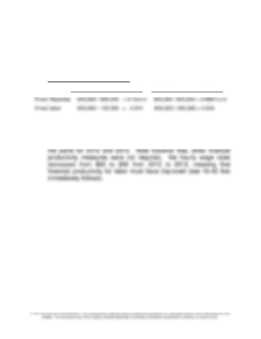
16–42 Partial Financial Productivity (30 min)
1.,2.,3. See spreadsheet solution below:
2013 2012
Units manufactured 600,000 800,000
Units of CT140 used 800,000 825,000
Number of labor hours used 150,000 200,000
Cost of CT140 per unit $156 $135
Direct labor wage rate per hour $56 $63
Total Materials Cost $124,800,000 =800,000 x $156 $111,375,000
Total Labor Cost $8,400,000 =150,000 x $56 $12,600,000
Total Materials and Labor Cost $133,200,000 $123,975,000
Financial Partial Productivity
Materials 0.004808 =600,000/124,800,000 0.007183
Labor 0.071429 =600,000/8,400,000 0.063492
Operational Partial Productivity
Materials 0.75000 =600,000/800,000 0.969697
Labor 4.00000 =600,000/150,000 4.000000
Current Output at Prior Year Productivity
Materials 618,750.00 =600,000/.969697
Labor 150,000.00 =600,000/4.0
Materials 800,000 618,750 618,750 825,000
Labor 150,000 150,000 150,000 200,000
Cost per unit of input
Materials $156 $156 $135 $135
Labor $56 $56 $63 $63
Direct materials 0.004808 (0.001408) 0.006216 (0.000967) 0.007183 – 0.007183 (0.002375)
Direct Labor 0.071429 – 0.071429 0.007937 0.063492 – 0.063492 0.007937
16–25
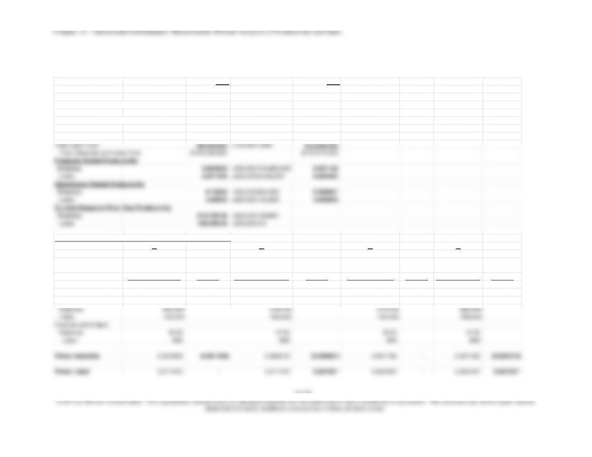
16-42 (continued-1)
1.
Financial Partial Productivity 2013 2012
Materials 0.004808 =600,000/124,800,000 0.007183
Labor 0.071429 =600,000/8,400,000 0.063492
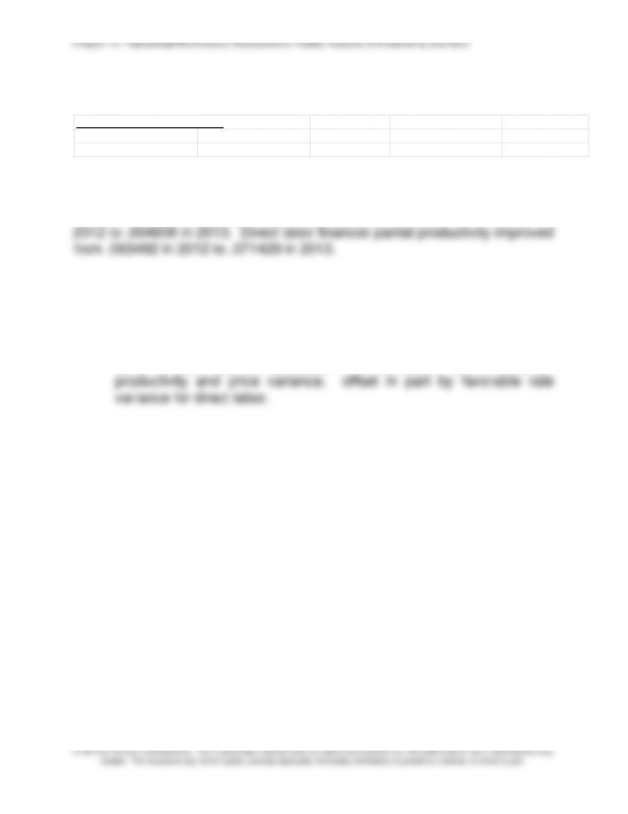
2.
Direct material financial partial productivity decreased from .007183 in
3.
The partial financial productivity ratios are calculated and compared in the
speadsheet above.
4. The decompositions suggest that changes in financial productivity from
2012 to 2013 can be attributed to unfavorable direct materials
16–26
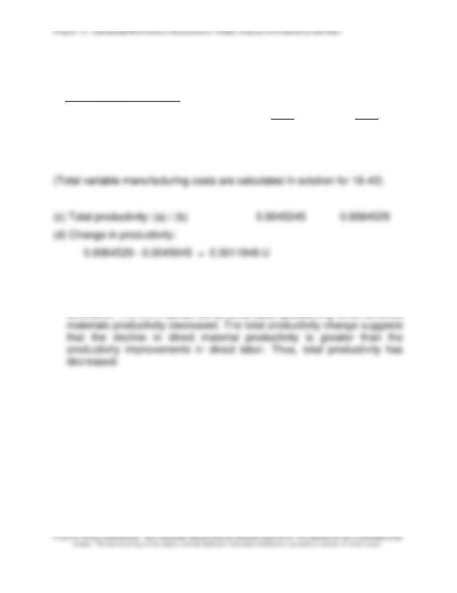
16–43 Total Productivity (15 min)
1. Total productivity in units
2013 2012
(a) Total units manufactured: 600,000 800,000
(b) Total variable manufacturing
costs incurred (see 16-42): $133,200,000 $123,975,000
2. Financial partial productivity measures indicate that the changes in
productivity for direct materials and direct labor are in opposite
directions. The firm maintained its direct labor productivity while its direct
16–27
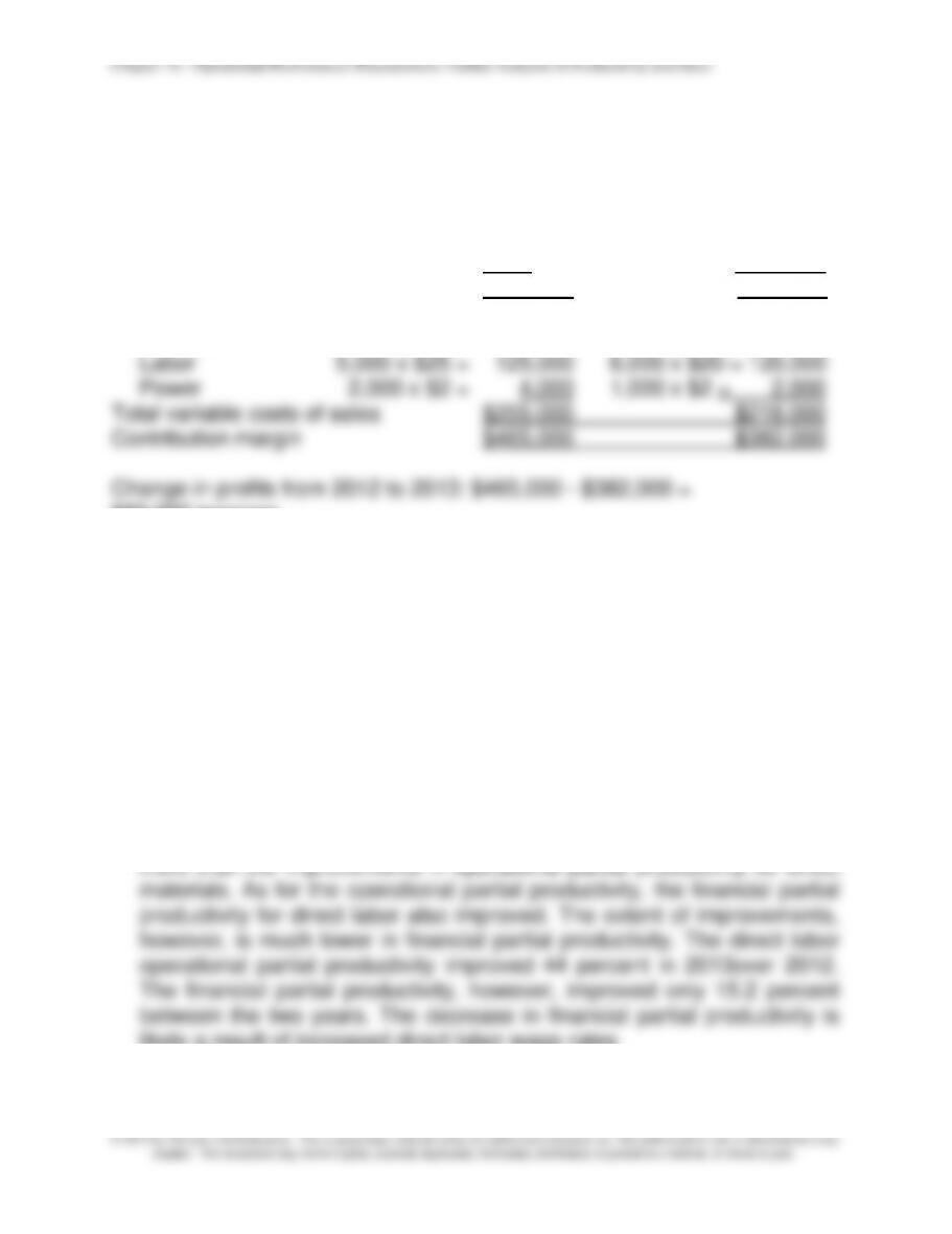
16–44 Operational and Financial Partial Productivity (45 min)
1. Simpson Company
Comparative Income Statement
For the years 2012 and 2013
2013 2012
Sales 18,000 x $40 = $720,000 15,000 x $40 =$600,000
Variable cost of sales:
Materials 12,600 x $10 = $126,000 12,000 x $8 = $96,000
$83,000 increase
2.3., See spreadsheet on following sheet.
4. Both direct materials and direct labor operational partial productivity
improved from 2012 to 2013. In 2013 the firm was able to manufacture
more output for each unit of materials placed into production and for
each hour used in production. The operational productivity of power in
2013 deteriorated from 2012. It is possible that the firm used more
equipment in production in 2013 which reduced consumption of
materials and production hours.
The financial partial productivity for both direct materials and power
deteriorated from 2012 to 2013. Increases in direct materials costs were
likely a result of increased direct labor wage rates.
Chapter 16 – Operational Performance Measurement: Further Analysis of Productivity and Sales
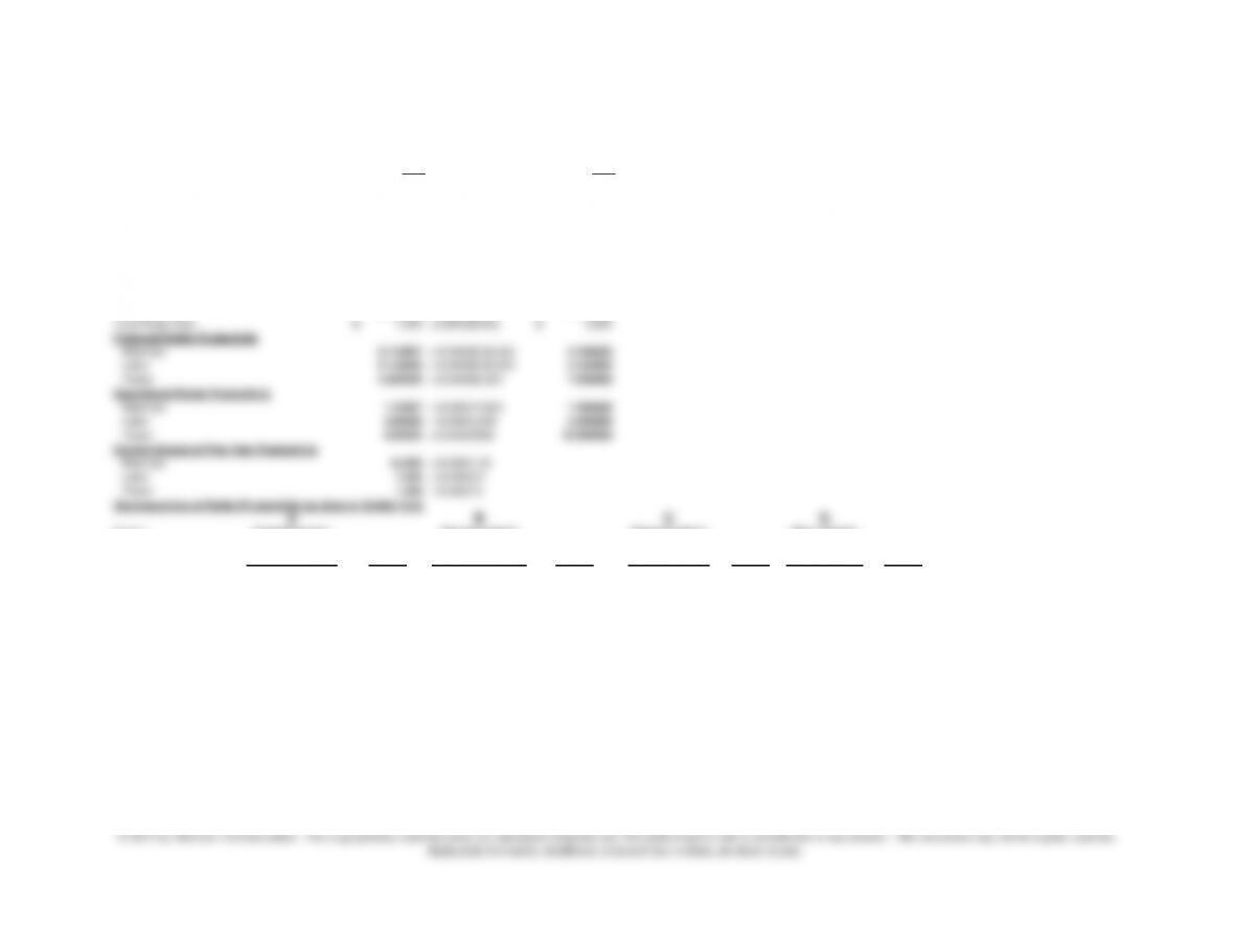
16–44 (continued –1)
2013 2012
Units manufactured 18,000 15,000
Materials used 12,600 12,000
Number of labor hours used 5,000 6,000
Cost of materials used per pound $10 $8
Direct labor wage rate per hour $25 $20
Power used (kwh) 2,000 1,000
Cost of power per kwh $2 $2
Total Materials Cost $126,000 =12,600x$10/lb $96,000
Total Labor Cost $125,000 =5,000x$25/hr $120,000
Total Power Cost 4,000$ =2,000x$2/kwh 2,000$
Financial Partial Productivity
Materials 0.142857 =18,000/$126,000 0.156250
Labor 0.144000 =18,000/$125,000 0.125000
Power 4.500000 =18,000/$4,000 7.500000
Operational Partial Productivity
Materials 1.42857 =18,000/12,600 1.250000
Labor 3.60000 =18,000/5,000 2.500000
Power 9.00000 =18,000/2000 15.000000
Current Output at Prior Year Productivity
Materials 14,400 =18,000/1.25
Labor 7,200 =18,000/2.5
Power 1,200 =18,000/15
Decomposition of Partial Productivity (as done in Exhibit 16.5)
Chapter 16 – Operational Performance Measurement: Further Analysis of Productivity and Sales
16–29
16-44 (continued –2)
5. See spreadsheet above.
6. Productivity for both direct materials and direct labor improved in 2013.
The percentages of improvements for 2013 over 2012 in productivity
are 11.43% (=.017857/.15625) and 35.2 (=.044/.125) for direct

Chapter 16 – Operational Performance Measurement: Further Analysis of Productivity and Sales
16–30
16-45 Operational and Financial Partial and Total Productivity (30 min)
1. Operational Partial Productivity
MF LI Difference
DM 20,000 / 300,000 = 0.0667 20,000 /200,000 = 0.1 0.0333 F*
DL 20,000 / 100,000 = 0.2 20,000/120,000= 0.1667 0.0333 U
* The direction of variances denotes the advantage of LI over MF.
It is not clear which is the better of the two approaches. The operational
partial productivity shows that LI has a higher productivity in direct
materials while MF yields a higher direct labor productivity.
2. Manufacturing Cost
MF LI
DM 20,000 /$2,400,000 = 0.0083 20,000/$1,600,000=0.0125 .0042 F
DL 20,000 /$2,500,000 = 0.008 20,000/$3,000,000=0.0067 .0013 U
3. Total Productivity