Unlock document.
This document is partially blurred.
Unlock all pages and 1 million more documents.
Get Access

Chapter 16 - Operational Performance Measurement: Further Analysis of Productivity and Sales
16-1
Chapter 16
Operational Performance Measurement: Further Analysis of
Productivity and Sales
Teaching Notes for Cases
Case 16-1 Dallas Consulting Group*
This case serves as a review of sales variances. Since all costs are fixed, it is unnecessary to do a variance
analysis based on contribution. Instead, the analysis is better done based solely on revenues. The variances
shown in Exhibit 1 are computed for the “levels” explained in the “Note on Managing Against Expectations.”
Students should recognize the following points:
1. Profit was $40,000 more than expected (Total Variance).
2. There was a total unfavorable Volume Variance of $42,000 due to the decline in the actual number of billed
hours (from 15,000 down to 14,000).
3. There was a favorable Mix Variance of 72,000 because of the shift in the product mix resulting in a higher
relative percentage of sales of the higher priced product (B) than expected (and a corresponding decrease in
the relative percentage sales of A).
4. There was a favorable Price Variance of $10,000 due to the increase in the rate charged for product A
(from $30 up to $35 per hour).
5. Product A:
1. Volume Variance is unfavorable due to the decline in the actual number of hours billed.
2. Mix Variance is unfavorable because of the decline in the number of hours billed for product A as a
percentage of total sales (from 40 percent down to 14 percent).
3. Price Variance is favorable because of the increase in the rate charged for product A (from $30 up to
$35 per hour).
6. Product B:
1. Volume Variance is unfavorable due to the decline in the actual number of hours billed.
2. Mix Variance is favorable because of the increase in the number of hours billed for product B as a
percentage of total sales (from 60 percent up to 86 percent).
3. Product B has no Price Variance since the actual billed rate was equal to the expected rate.
7. The total market decline of 3,000 hours (from 115,000 hours down to 112,000 hours) caused DCG to lose
$159,600 of revenue (opportunity loss?) based on their expected market share of 10 percent.
8. By increasing its market share form 10 percent to 12.5 percent, DCG increased revenues by $117,600.

Chapter 16 - Operational Performance Measurement: Further Analysis of Productivity and Sales
16-2
EXHIBIT 1
Operating Income Variance:
Original Budget $630,000
Actual Results 670,000
Total Variance $ 40,000
Sales Volume Variance:
Original Budget $630,000
Flexible Budget 660,000
Volume and Mix Variance $ 30,000
Selling Price Variance:
Flexible Budget $660,000
Actual Results 670,000
Price Variance $ 10,000
Sales Mix and Sales Quantity Variances:
(AV = Actual Volume, SV = Standard Volume,
AM = Actual Mix, SM = Standard Mix,
AP = Actual Price, SP = Standard Price)
Original Budget $630,000 (SV, SM, SP)
Adj. Flexible Budget 558,000 (AV, SM, SP)
Sales Quantity Variance $ 42,000 Unfavorable
Adj. Flexible Budget $558,000 (AV, SM, SP)
Flexible Budget 660,000 (AV, AM, SP)
Mix Variance $ 72,000 Favorable
Market Share and Market Size Variances:
Original Budget $630,000 (SV, SM, SP)
Forecasted Market Share 470,400 (Act. Mkt., Expected Share, SM, SP)
Overall Market Variance $159,600 Unfavorable
Forecasted Market Share $470,400 (Act. Mkt., Expected Share, SM, SP)
Adj. Flexible Budget 588,000 (AV, SM, SP)
Market Share Variance $117,600 Favorable
By Product ($ Thousands);
Product Vol. Mix Mix Price Total
A 12 U 108 U 120 U 10 F 110 U
B 30 U 180 F 150 F 0 150 F
Total 24 U 72 F 32 F 10 F 40 F
Chapter 16 - Operational Performance Measurement: Further Analysis of Productivity and Sales
16-3
Teaching Strategies for Articles
16-1 Anthony J. Hayzen and James M. Reeve: “Examining the Relationships in Productivity
Accounting”
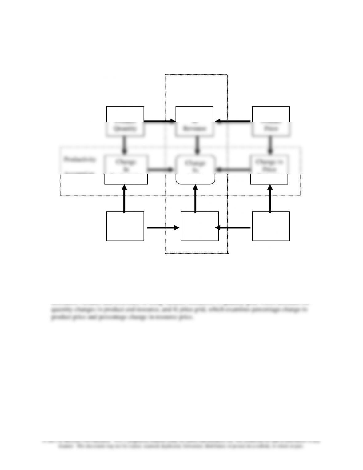
Change in profit of a firm or business unit can be analyzed in terms of a change in productivity and a
change in price recovery. Change in product quantities and change in resource quantity drive the change
in productivity. Change in product prices and change in resource prices drive the change in price
recovery. These relationships can be displayed to provide an instant visual analysis of the causes of profit
change. Such visualization can provide a robust method for analyzing strategy and stakeholder
relationships.
Discussion questions:
1. What is productivity accounting?
2. How can productivity accounting guide the overall strategy of the firm?
3. Give an example showing that a traditional business performance indicator may give conflicting
signals on a firm's performance.
Traditional business measures for performance include such measures as profit and sales per
square yard. Let’s assume that, in 2009, Alice sold 100 units at $80 each, paid $40 per unit to Bobby
for the merchandise and $2,000 to Centry Properties to rent 50 square yards of retail space. Alice also
2009 2010
Sales $8,000 $9,600
Cost of Goods Sold 4,000 4,800
Sales per square yard increased from $160 to $192 while the operating income decreased from $2,000
to $1,800.
4. What are the elements in using productivity accounting to evaluate changes in profits?
Productivity accounting explains changes in profit as a function of changes in productivity and
changes in price recovery as shown below.
Chapter 16 - Operational Performance Measurement: Further Analysis of Productivity and Sales
16-4
Where: Change in Productivity = Output Quantity/Input Quantity, and
Price Recovery = Output Price/Input Price
These relationships are depicted in a nine-box diagram:
Traditional Measure
Accounting
5. What grid diagrams are needed in order to have an overall picture of the business's performance?
A firm is likely to need four grid diagrams to explain a change in it performance. These four grids
are 1) profit grid that explains profit changes in terms of productivity variance and price recovery
variance, 2) productivity grid, which accounts for change in productivity by looking at capacity
utilization variance and efficiency in using variance resources, 3) quantity grid, which accounts for
Change in
Change
Change in
In
Productivity
Price
Recovery
Change in
Resource
Quantity
Change
In
Cost
Change in
Resource
Price
In
Profit
Chapter 16 - Operational Performance Measurement: Further Analysis of Productivity and Sales
16-5
16-2: “Lean Accounting: What’s it All About?”
This article provides and introduction and illustration of the concept of lean accounting. A key ideas is
the role of value streams. The illustration is based on an actual company, which is given the disguised
name MIP.
Discussion Questions:
1. Why lean accounting?
The move to lean accounting at MIP was motivated by three main concerns. One, the variance
data created by the accountants was dated and therefore of limited usefulness to managers. Two, the
information from the accountants provided the wrong incentives for managers. Three, the accounting
2. What are the five steps of the lean thinking model?
1. define value, especially with respect to customer value
2. identify the value stream, how value is produced for customers
3. What four areas did MIP address in implementing lean accounting?
1. performance measurement, in linking strategy to compensation and performance measurement
2. transaction elimination
4. How is waste defined in lean accounting?
Waste is defined, much as it is in the Toyota Production System, as:


