Chapter 15 – Operational Performance Measurement: Indirect-Cost Variances and Resource-Capacity Management
15–74
15–52 (Continued-2)
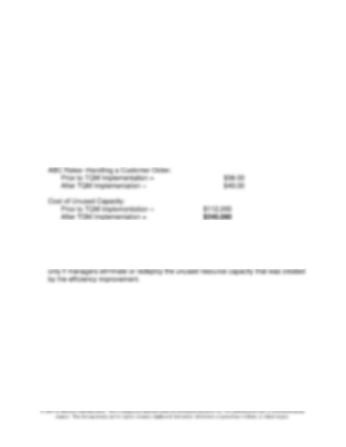
efficiency of the customer order-handling process. (Note: this cost might increase a
bit to cover the cost of the TQM initiative.)
Note, however, that the cost of unused capacity increases, from $112,000 (80%
capacity utilization) to $240,000 (57.14% capacity utilization).
Practical Capacity:
Prior to TQM Implementation = 10,000
After TQM Implementation = 14,000
Resource Cost (Handling Customer Orders) = $560,000
Budgeted # of Customer Orders = 8,000
Capacity Utilization:
Prior to TQM Implementation = 80.00%
After TQM Implementation = 57.14%
Conclusion: Efficiency initiatives (e.g., TQM) will lead to reduce resource spending
5. Faced with unused capacity, for example, the company can:
(1) Reduce spending on resources for the support activity in question, or
(2) Find ways to utilize existing, but currently unused, capacity (e.g., new-product
introduction)
Chapter 15 – Operational Performance Measurement: Indirect-Cost Variances and Resource-Capacity Management
15–75
6. Logically, we would assign to a given customer or market segment the cost of
unused capacity IF the associated capacity were acquired specifically to serve that
customer or market segment. IF the unused capacity is associated with a given
product line, then the cost of unused capacity should logically be assigned to that
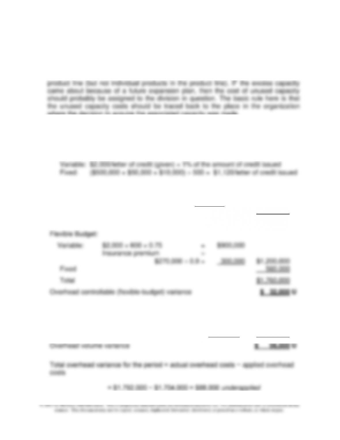
where the decision to acquire the associated capacity was made.
15–53 Two-Variance Analysis: Service Company Example (30 minutes)
1. Budgeted number of letters of credit approved: $1,000,000 $2,000 = 500
Overhead application rates:
2. Actual overhead costs incurred:
Variable: $2,000 × 600 × 0.75 × 110% = $990,000
Insurance premium 270,000 $1,260,000
Fixed: $560,000 × 95% = 532,000
Total $1,792,000
Flexible-budget: $1,760,000
Overhead applied $3,120 × 600 × 0.75 = $1,404,000
$2,700 ÷ (1 − 0.10) = 300,000 1,704,000
15–76
15–54 ABC versus Traditional Approaches to Control of Batch-Related Overhead
Costs (50-60 minutes)
Additional information needed to solve this problem (highlighted in bold):
Budgeted Actual
Results Results
Units produced and sold 10,000 9,000
Batch size (units) 250 200
No. of batches 40 45
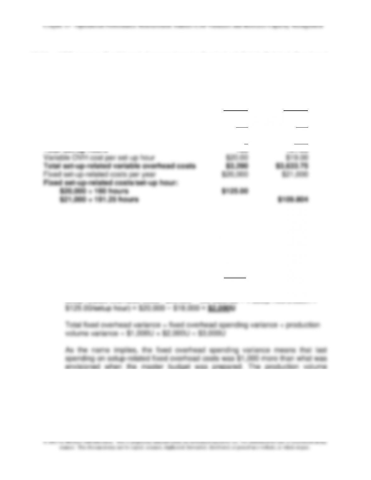
Set-up hours per batch 4 4.25
Note that the control (flexible) budget for set–up-related variable overhead costs should
be based in this case on set-up hours (the controllable factor). Thus, given an output
last year of 9,000 units, the company should have used 36 batches (9,000 units ÷ 250
units per batch). At a standard of 4.0 set-up hours per batch, the 9,000 units produced
equates to 144 set-up hours.
(1) (a) Fixed overhead spending variance = Actual fixed setup-related costs – budgeted
fixed setup-related costs = $21,000 − $20,000 = $1,000U
(b) Production volume variance = budgeted fixed setup-related costs – applied fixed
setup-related overhead costs= $20,000 − (36 batches × 4 setup-hours/batch ×
variance in this context means that capacity, measured in terms of budgeted
setup hours, was not fully utilized during the period. Specifically, the standard
allowed setup hours (for this year’s production), 144, was 16 less than capacity
available (160 hours). Thus, $2,000 = 16 hours × $125/hour.
Chapter 15 – Operational Performance Measurement: Indirect-Cost Variances and Resource-Capacity Management
15–77
15–54 (Continued-1)
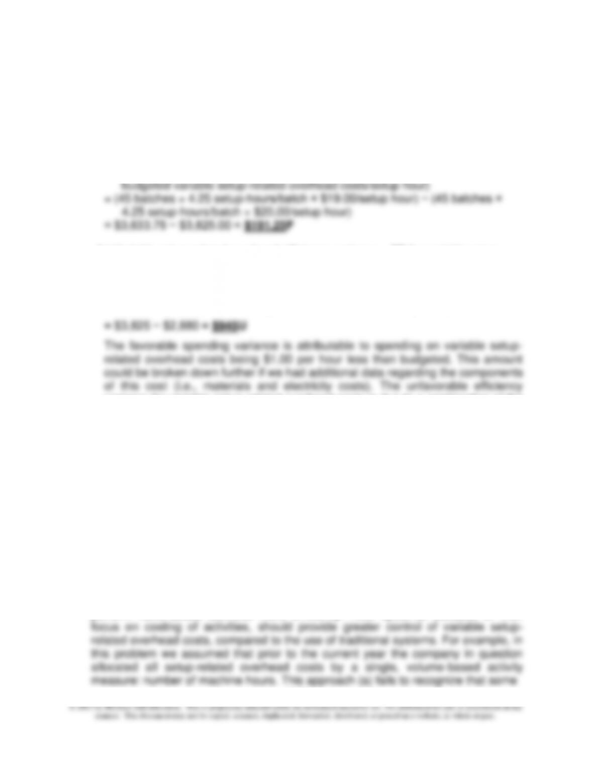
(2) (a) Variable setup-related overhead spending variance = actual variable setup–
related overhead costs − budgeted variable setup-related overhead costs based
on inputs (i.e., based on actual setup hours worked during the year)
= (actual batches × actual setup hours/batch × actual variable setup-related
overhead costs/setup hour) − (actual batches × actual setup hours/batch ×
(b) Variable setup-related overhead efficiency variance = FB for variable setup–
related overhead costs based on Inputs − FB for variable setup-related
overhead costs based on Outputs
= $3,825 − (36 batches × 4 setup-hours/batch × $20.00/setup hour)
variance for variable setup-related overhead costs is due to a combination of the
following two factors: (1) the actual output of the period (9,000 units) took 9 more
batches than standard (actual # of batches = 45; standard allowed batches = 36,
as shown above); and (2) each setup took slightly more time than standard (4.25
hours/setup vs. 4.00 hours/setup). The net unfavorable variable setup-related
overhead variance indicates that the favorable spending variance was not
enough to offset the unfavorable efficiency variance.
(3) Fixed setup-related overhead costs are controlled primarily prior to the point of
operations. That is, they are controlled primarily through the planning process (for
example, the capital budgeting process or the use of zero-based budgeting). These
costs basically relate to the capacity/ability to produce.
On the other hand, variable setup-related costs, by definition, vary in response to
one or more underlying causal factors (cost drivers). Therefore, these costs are
controlled by attempting to identify and eliminate non-value-added activities and to
perform value-added activities more efficiently. ABC systems, because of their
Chapter 15 – Operational Performance Measurement: Indirect-Cost Variances and Resource-Capacity Management
15–78
15–54 (Continued-2)
of these overhead costs are capacity-related and therefore controlled differently,
and (b) fails to identify meaningful strategies for cost control. When machine hours
are used as the basis for cost allocation and some costs (as in this case) are not
related to machine hours, then the variable overhead spending variance based on
machine hours will include the effect of spending on these other activities—in other
(4) Most companies find that a comprehensive control system consists of both financial
and nonfinancial performance indicators. Thus, one would expect that operating
units in the Bangor Manufacturing Company would have timely access to
nonfinancial performance indicators such as process yields (e.g., ratio of good
outputs to inputs), manufacturing processing time, reject rates, percent first-pass
yield, defect rates (e.g., parts-per-million, ppm), etc. Such information has the
advantage of being expressed in a manner that is readily interpretable by operating
personnel. As well, these data direct worker attention to actionable steps when a
Chapter 15 – Operational Performance Measurement: Indirect-Cost Variances and Resource-Capacity Management
15–79
15–55 Decision-Making under Uncertainty (Appendix) (30-40 minutes)
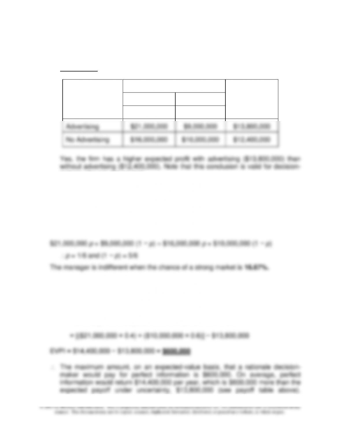
1. Payoff Table
Possible
Courses of
Action
State of the Market
Expected
Value of Each
Action
Strong
Weak
Prob. = 0.4
Prob. = 0.6
Advertising
$21,000,000
$9,000,000
$13,800,000
No Advertising
$16,000,000
$10,000,000
$12,400,000
Yes, the firm has a higher expected profit with advertising ($13,800,000) than
without advertising ($12,400,000). Note that this conclusion is valid for decision–
makers who are risk-neutral.
2. Let p be the probability that the market is strong; thus, the probability that the market
is weak is 1 − p.
At the indifference point:
E(Advertising) = E(No Advertising)
3. The Expected Value of Perfect Information (EVPI) = maximum value the manager
would pay to have knowledge (i.e., certainty) of the revealed state of nature.
EVPI = Expected (i.e., long-run average) profit with perfect information − expected
(i.e., long-run average) profit without perfect information
Chapter 15 – Operational Performance Measurement: Indirect-Cost Variances and Resource-Capacity Management
15–80
15–56 Variance Investigation under Uncertainty (Appendix) (30-40 minutes)
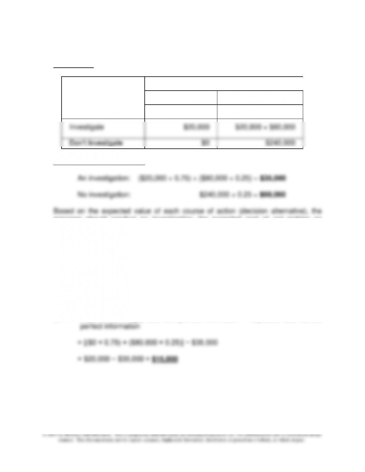
1. Payoff Table
Courses of Action
States of Nature
In-Control
Out-of-Control
(1 − p) = 0.75
p = 0.25
Investigate
$20,000
$20,000 + $60,000
Don’t Investigate
$0
$240,000
2. Expected cost of conducting:
manager should conduct an investigation: the expected cost of not making an
investigation > expected cost of conducting an investigation.
3. The Expected Value of Perfect Information (EVPI) = maximum value the manager
would pay to have knowledge (i.e., certainty) of whether the process is in control or
out of control. In this decision context, the EVPI can be thought of as the difference
between the expected cost with perfect information and the expected cost without
perfect information. (To calculate the former, we need to choose for each possible
state of nature the best course of action [decision] and then multiply the associated
“cost” by the probability of that state of nature occurring. We then sum these resulting
expected costs to get the expected cost with perfect information.)
EVPI = expected (average) cost with perfect information − expected cost without
Chapter 15 – Operational Performance Measurement: Indirect-Cost Variances and Resource-Capacity Management
15–81
15–57 All Manufacturing Variances (50–60 minutes)
1. At the time of purchase. Recording the price variance for materials at time of
purchase recognizes the variance at the point it occurs. Further, if the organization in
question uses a standard cost system, then this practice results in the materials
inventory being carried at standard cost, which is consistent with the way WIP
Inventory and Finished Goods Inventory are carried. Finally, recognizing the price
variance at point of purchase provides management with timely information that,
presumably, can be used to correct any problems that arise.
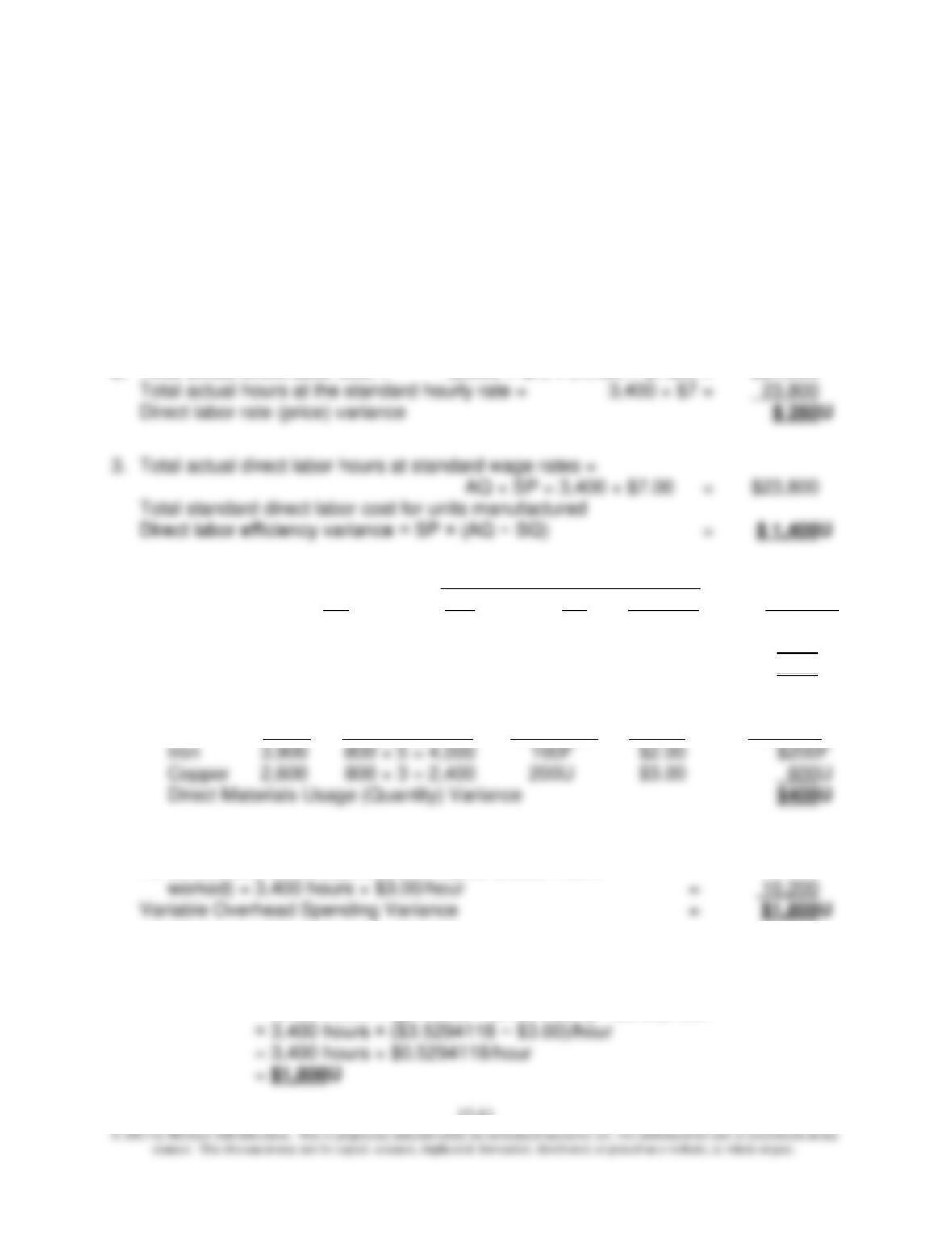
2. Total actual direct labor cost = (2,000 × $7) + (1,400 × $7.20) = $24,080
4. Price Price
AQ AP SP AP − SP Variance
Iron 5,000 $2 $2 – 0 – – 0 –
Copper 2,200 $3.10 $3 $0.10 $220
Direct Materials purchase price variance $220U
5. Usage
AQ SQ (AQ − SQ) SP Variance
6. Actual variable overhead (given) = $12,000
FB for Variable Overhead based on Inputs (actual hours
Alternative formula for variable overhead spending variance:
Variance = AQ × (AP − SP)
= 3,400 hours × ([$12,000 ÷ 3,400 hours] − $3.00)/hour
Chapter 15 – Operational Performance Measurement: Indirect-Cost Variances and Resource-Capacity Management
15–82
15–57 (Continued)
7. FB for Variable Overhead based on Inputs (i.e., based on actual
hours worked—see 6 above) = $10,200
Total standard variable overhead applied for units
8. Actual fixed overhead (given) $8,800
9. Budgeted fixed overhead (see 8 above) $8,000
Fixed overhead applied to units manufactured
Variance = SP × (Denominator volume − Actual Units Produced)
= $8.00/unit × (1,000 units − 800 units) = $1,600U
Chapter 15 – Operational Performance Measurement: Indirect-Cost Variances and Resource-Capacity Management
15–83
Check Figures
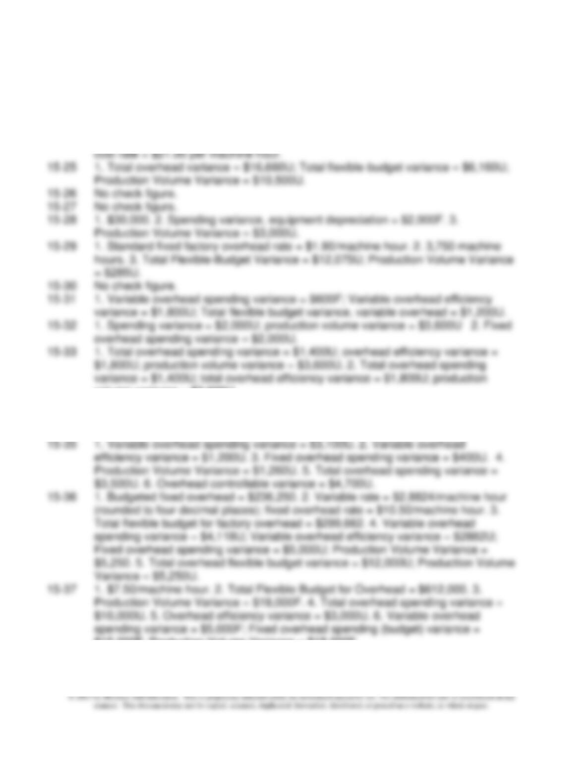
15–24 1. At 4,000 machine hours, budgeted variable overhead = $84,000; budgeted fixed
overhead = $65,500; at 5,000 machine hours, budgeted variable overhead =
$105,000; budgeted fixed overhead = $65,500. 2. Estimated variable overhead
volume variance = $3,600U
15–34 1. Total flexible budget (controllable) variance = $3,200U; production volume
variance = $3,600U 2. Flexible budget variance = $3,200U; production volume
variance = $3,600U
$15,000F; Production Volume Variance = $18,000F.
15–38 1. Total overhead spending variance = $24,200U; Total Overhead Efficiency
Variance = $23,800U. 2. Total overhead spending variance = $32,200U; Total
Chapter 15 – Operational Performance Measurement: Indirect-Cost Variances and Resource-Capacity Management
15–84
overhead efficiency variance = $19,800U. 3. Total overhead spending variance =
$14,000U; Total overhead efficiency variance = $38,000U.
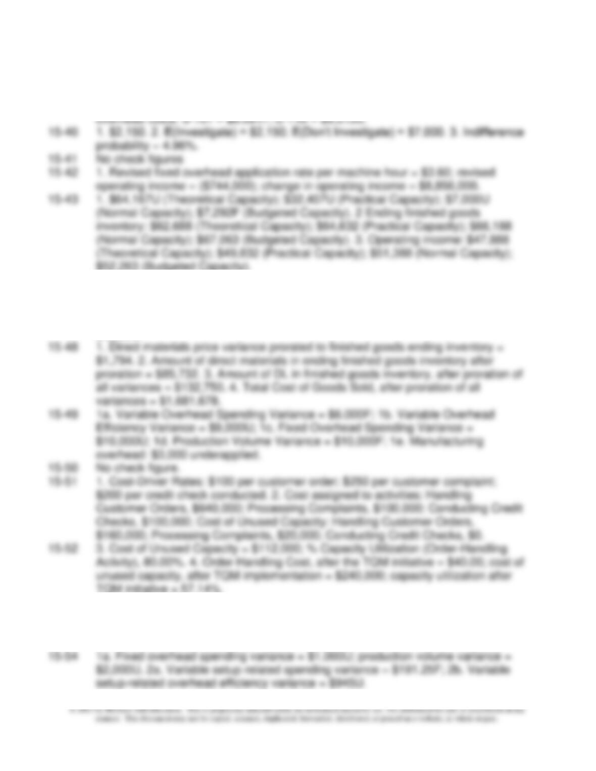
15–39 1. Budgeted cost per unit, S-101= $7.1535; C-110 = $10.11.61. 2. Allocated
$52,263 (Budgeted Capacity).
15–44 No check figure.
15–45 No check figure.
15–46 No check figure.
15–47 1a. 396,000; 1b. $33,000U; 1c. $22,000U; 1d. $25,000F; 1e. $594,000; 1f.
$6,000U.
TQM initiative = 57.14%.
15–53 1. Budgeted overhead application rates: variable overhead = $2,000/letter of credit
(given) + 1% of the amount of credit issued; fixed overhead = $1,120/letter of credit
issued. 2a. Total Overhead Controllable (Flexible-Budget) Variance = $32,000U;
2b. Overhead volume variance = $56,000U.
Chapter 15 – Operational Performance Measurement: Indirect-Cost Variances and Resource-Capacity Management
15–85
15–55 1. E(Advertising) = $13,800,000; E(No Advertising) = $12,400,000. 2. Indifference
probability = 16.67%. 3. EVPI = $600,000.
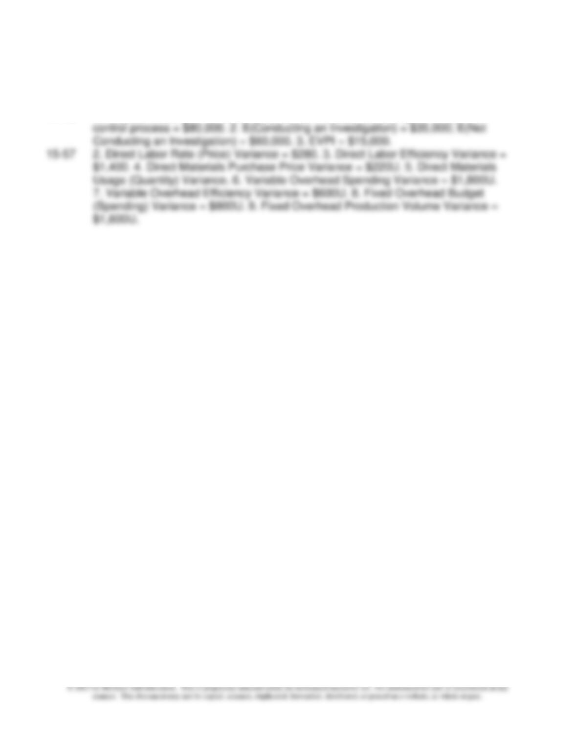
15–56 1. Payoffs: Investigate an in-control process = $20,000; Investigate an out-of–