Chapter 14 – Operational Performance Measurement: Sales, Direct-Cost Variances, and the Role of Nonfinancial
Performance Measures
14–31
14-36 Ethical Considerations (20-25 minutes)
1. The IMA Statement of Ethical Professional Practice provides a set of four overarching
principles designed to guide member behavior. As well, there is an expectation that
IMA members “encourage others within their organization to adhere to the principles
of honesty, fairness, objectivity, and responsibility.”
In the present case, however, we focus on the ethical standards related to the
behavior of the Purchasing Manager:
▪ Competence: the “reporting” of sub-standard purchase prices for raw materials
(represented by sub-standard materials) violates the expectation that decision–
price. The expected negative results associated with the use of the sub-standard
materials is the key issue.
▪ Credibility: the purchasing manager, working with the cost accountant, in this
case has a responsibility to ensure that information is communicated fairly and
objectively. Further, this standard requires the disclosure of all relevant
information that could reasonably be expected to influence a user’s
understanding of any resulting reports or analyses, such as the standard cost
variance information related to the purchasing transaction.
2. The IMA Standards of Ethical Professional Practice indicate that in resolving ethical
conflicts the accountant should first act in accordance with the organization’s
established policies regarding the resolution of such conflicts. If this step does not
resolve the issue, the accountant should then discuss the issue with his/her
immediate supervisor, which in this case could be the controller of the organization.
If, after such consultation, resolution cannot be reached, the individual should
Chapter 14 – Operational Performance Measurement: Sales, Direct-Cost Variances, and the Role of Nonfinancial
Performance Measures
14–32
raised, then it might be appropriate at a certain point for the accountant to make
contact with an outside authority.)
14–37 Standard Costs and Ethics (15 Minutes)
As controller of the company, Mary’s behavior is not ethical. Under the Credibility
standard, Mary has an obligation to communicate information fairly and objectively.
Further, under the Credibility standard she has a responsibility to prepare complete
and clear reports and recommendations. That is, she must disclose the price
versus loyalty to the company for which she works) by: (1) not being the person who
sets the standard cost for the apple juice, and (2) not restricting source of supply
(e.g., by mandating that apple juice must be purchased from her friend’s business).
14–38 Journal Entries (10-15 minutes)
Oct. 7 Materials Inventory (720 lbs. × $40/lb.) 28,800
Materials Purchase-Price Variance—PVC (720 lbs.× $1/lb.) 720
Issued 720 pounds of PVC for the production of 780 units of XV-1. Standard
usage is 1 lb. per unit of XV-1, at $40 per pound.
Chapter 14 – Operational Performance Measurement: Sales, Direct-Cost Variances, and the Role of Nonfinancial
Performance Measures
14–33
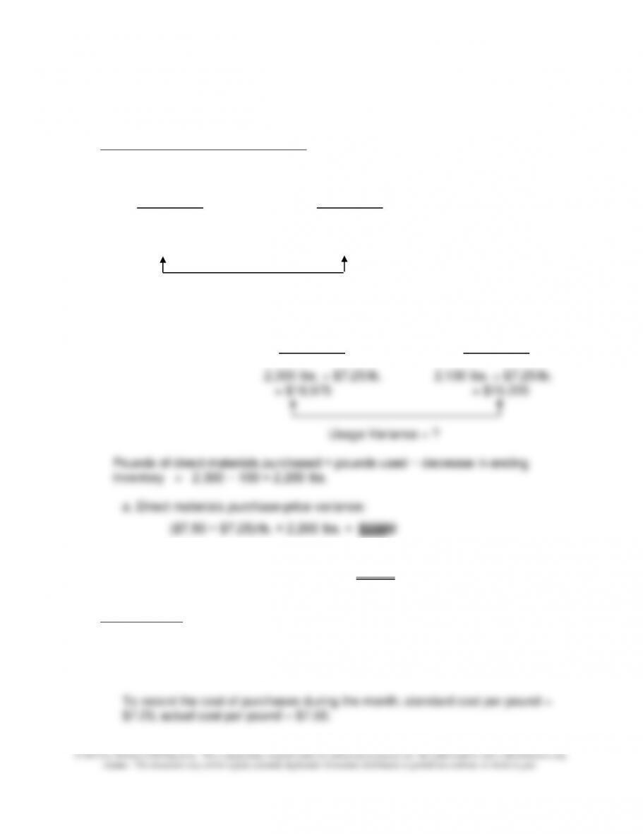
14–39 Direct Materials Variances—Journal Entries (20-25 minutes)
1. Determination of variances for March:
Actual Purchases Actual Purchases
at Actual Cost at Standard Cost
(AQ) × (AP) (AQ) × (SP)
(AQ) × $7.50/lb. (AQ) × $7.25/lb.
= ? = ?
Purchase-Price Variance = ?
Actual Usage at Flexible-Budget
Standard Cost Amount
(AQ) × (SP) (SQ) × (SP)
b. Direct materials usage variance:
(2,300 − 2,100) lbs. × $7.25/lb. = $1,450U
2. Journal entries:
Materials Inventory 15,950
Materials Purchase-Price Variance 550
Accounts Payable 16,500
Chapter 14 – Operational Performance Measurement: Sales, Direct-Cost Variances, and the Role of Nonfinancial
Performance Measures
14–34
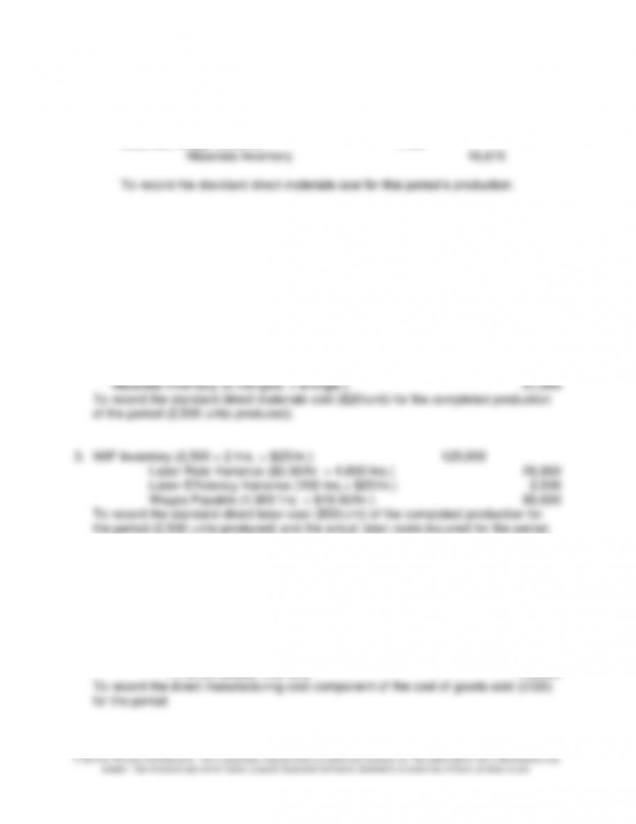
14–39 (Continued)
WIP Inventory 15,225
Materials Usage Variance 1,450
14-40 Standard Costing and Journal Entries (30 minutes)
1. Materials Inventory (6,000 gals. × $10.00/gal.) 60,000
Materials Purchase-Price Variance 2,700
Accounts Payable (6,000 gals. × $10.45/gal.) 62,700
To record, on open account, direct materials: 6,000 gals. @ standard cost of
$10.00/gal. Actual cost per gallon = $10.45.
2. WIP Inventory (2,500 × 2 gals. × $10/gal.) 50,000
Materials Usage Variance (100 gals. × $10/gal.) 1,000
4. Finished Goods Inventory ($70 × 2,500 units) 175,000
WIP Inventory 175,000
To record the direct manufacturing cost component of cost of goods manufactured
for the period.
5. CGS ($70/unit × 2,000 units) 140,000
Finished Goods Inventory 140,000
Chapter 14 – Operational Performance Measurement: Sales, Direct-Cost Variances, and the Role of Nonfinancial
Performance Measures
14–35
6. Accounts Receivable ($150/unit × 2,000 units) 300,000
14–41 Control of Operating Processes/Non-financial Performance Indicators (30-
45minutes)
1. Organizations engage in a variety of processes in order to deliver the stated value
proposition to its targeted customers and in order to achieve its stated financial
objectives. These processes, for expository purposes, might be grouped into the
following: (a) operating processes, (b) customer-management processes, (c) growth
and innovation processes, and (d) social and regulatory processes.
Operating processes might be defined as what the organization does, on a day-to–
day basis, to produce and deliver to customers its outputs (services and/or products).
Thus, operating processes include activities such as: acquiring raw materials from
supplier firms; producing finished goods and services; and, distributing the finished
advantage.) Growth and innovation processes might be further subdivided into the
following four categories: (1) identifying opportunities for new products and services—
that is, generating new ideas; (2) managing the organization’s R&D portfolio; (3)
designing and developing new products and services—the core of product
development; and, (4) bringing new products and services to market. Social and
2. The following are examples of possible objectives and associated performance
indicators for two operating processes: production, and distribution.
Chapter 14 – Operational Performance Measurement: Sales, Direct-Cost Variances, and the Role of Nonfinancial
Performance Measures
14–36
Production Process
(1) Achieve Reduction in the Cost of Outputs (Products and/or Services)
14–41 (Continued-1)
• Total Cost of Quality (COQ), over time
• Ratio of Prevention + Appraisal Costs to Internal + External Failure Costs
• Total Cost of Quality (COQ), as a percentage of:
o Sales Revenue
• Processing (Manufacturing) Time (i.e., time actually used for processing; it
excludes “non-value-added” time such as wait time, movement, and set-
up time)
(4) Improve the Utilization of Capital (Fixed) Assets
• Number and % of machine breakdowns
• Manufacturing Flexibility (e.g., number of products or services that the
facility in question can produce and deliver to customers)
Chapter 14 – Operational Performance Measurement: Sales, Direct-Cost Variances, and the Role of Nonfinancial
Performance Measures
14–37
Distribution Process
(1) Reduce Cost of Servicing Customers
• Activity-based costs associated with key activities (e.g., storage and
delivery to customers)
• lead time, from placement of orders to delivery of product/service
14–41 (Continued-2)
Enhance Quality of the Distribution Process
• % of items delivered on or before scheduled delivery
•
14-42 JIT and Process Cycle Time Efficiency (PCE) (45–50 minutes)
1. The terms “value–added” and “non-value-added” are defined from the perspective of
the customer (i.e., an external perspective is taken). Because the perspective is
external, the notions of “value-added” vs. “non-value-added” are not strictly or
uniquely defined. The key question in classifying activities is whether the consumer
would “pay” for the activity. This is one way to operationalize the two terms. We note
production time (i.e., time expended for the product to be made). Excluded from this
measure are “non-value-added” times associated with moving, storing, or inspecting
the product. A measure of processing time efficiency is called “processing cycle
efficiency (PCE),” which is defined as follows:
Chapter 14 – Operational Performance Measurement: Sales, Direct-Cost Variances, and the Role of Nonfinancial
Performance Measures
14–38
PCE = “Value–Added Time” ÷ “Total Manufacturing Cycle Time”
or,
PCE = Processing Time ÷ (Processing Time + Moving Time + Storage Time +
Inspection Time)
2. Cycle time is the total time required from the start of production to completion of
outputs. Process (or processing or manufacturing) time represents the time actually
(cycle) time (time between when an order is received by manufacturing and the time
that order is completed), and delivery time (time between when an order is completed
and when that order is received by the customer). As shown in Exhibit 14.14, we
might further break-down manufacturing lead (cycle) time into waiting time and
manufacturing (or, production cycle) time. Finally, manufacturing time can be
decomposed into the elements reflected above in the formula for PCE.
Chapter 14 – Operational Performance Measurement: Sales, Direct-Cost Variances, and the Role of Nonfinancial
Performance Measures
14–39
14-42 (Continued)
3. Processing Cycle Efficiency (PCE), Pre-JIT:
PCE = 1.0 hr. ÷ (1.0 hr. + 1.0 hr. + 0.50 hr. + 0.75 hr.)
= 1.0 ÷ 3.25
= 30.77%
Alternatively, 60 minutes ÷ 195 minutes = 30.77%.
Processing Cycle Efficiency (PCE), Post-JIT Implementation:
Alternatively, 30 minutes ÷ 80 minutes = 37.50%.
4. Percentage Improvement, Pre-JIT versus Post-JIT Implementation:
% change = (0.375 − 0.3077) ÷ 0.3077 = 22% (actual amount is 21.87%)
5. The move to a JIT manufacturing process should be accompanied by improvements
in quality, reductions in waste and inefficiencies, reduction in inventories held,
improvements in cycle times (and customer response time, CRT), and, perhaps,
• % of defects, incoming orders (supplies, materials, and subassemblies)
• % of suppliers that are certified (i.e., who are qualified to deliver without
incoming inspections)
Chapter 14 – Operational Performance Measurement: Sales, Direct-Cost Variances, and the Role of Nonfinancial
Performance Measures
14–40
Production-Related Measures
• parts-per-million (ppm) defect rates
• machine uptime
14-42 (Continued)
• % capacity utilization (i.e., managing the supply of resource capacity)
• actual production as % of planned production
Distribution Activities
• % of items delivered with no (zero) defects
Chapter 14 – Operational Performance Measurement: Sales, Direct-Cost Variances, and the Role of Nonfinancial
Performance Measures
14–41
PROBLEMS
14–43 Master Budget, Flexible Budget, and Profit-Variance Analysis; Spreadsheet
Application (75–90 minutes)
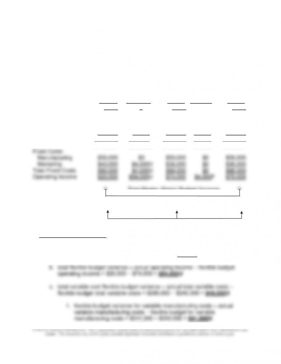
1.
Flexible- Sales Master
Actual Budget Flexible Volume (Static)
Results Variances Budget Variance Budget
Unit sales 4,000 0 4,000 100F 3,900
Sales $390,000 $10,000U $400,000 $10,000F $390,000
Variable Costs:
Manufacturing $241,000 $41,000U $200,000 $5,000U $195,000
Marketing $39,000 $1,000F $40,000 $1,000U $39,000
Total Variable Costs $280,000 $40,000U $240,000 $6,000U $234,000
CM $110,000 $50,000U $160,000 $4,000F $156,000
Total Master (Static) Budget Variance
$50,000U
Flexible-Budget Sales Volume
Variance Variance
$54,000U $4,000F
2. Profit-variance components:
a. total master (static) budget variance = actual operating income − master
budget operating income = $20,000 − $70,000 = $50,000U
Chapter 14 – Operational Performance Measurement: Sales, Direct-Cost Variances, and the Role of Nonfinancial
Performance Measures
14–42
14–43 (Continued-1)
2. flexible-budget variance for variable nonmanufacturing costs = actual
variable nonmanufacturing costs − flexible-budget variable
nonmanufacturing costs = $39,000 − $40,000 = $1,000F
d. total fixed cost flexible-budget variance = actual total fixed costs − flexible–
budget total fixed costs = $90,000 − $86,000 = $4,000U
1. flexible-budget variance for fixed manufacturing costs = actual fixed
manufacturing costs − flexible-budget for fixed manufacturing costs =
3. Interpretation of profit variances:
a. total master (static) budget variance: this is the total operating-profit variance
for the period, i.e., the difference between actual operating profit and operating
profit as stated in the master (static) budget. Notice that this variance is a function
explained below.
b. total flexible-budget variance: this variance explains the portion of the total
profit variance for the period related to a combination of three factors: selling
price per unit, variable cost per unit, and total fixed costs. These variances, and
As such, it can be further decomposed into a total variance for direct
materials, a total variance for direct labor, and a total variance for variable
overhead (the latter of which is covered in Chapter 15).
Chapter 14 – Operational Performance Measurement: Sales, Direct-Cost Variances, and the Role of Nonfinancial
Performance Measures
14–43
14–43 (Continued-2)
2. flexible-budget variance for total variable nonmanufacturing costs: this
variance represents the portion of the flexible-budget variance that is
attributable to nonmanufacturing cost per unit being different from budgeted
amount. As such, it can be further decomposed into a total variance for
each nonmanufacturing cost element (e.g., selling expenses).
d. flexible-budget variance for total fixed costs: this variance is also referred to
as a spending variance, since it represents the difference between actual fixed
costs and budgeted fixed costs. As such, the variance can be further broken
down into functional categories, as explained below.
1. flexible-budget variance for total fixed manufacturing costs: this is the
portion of the flexible-budget variance for total fixed costs that is attributable
14–44
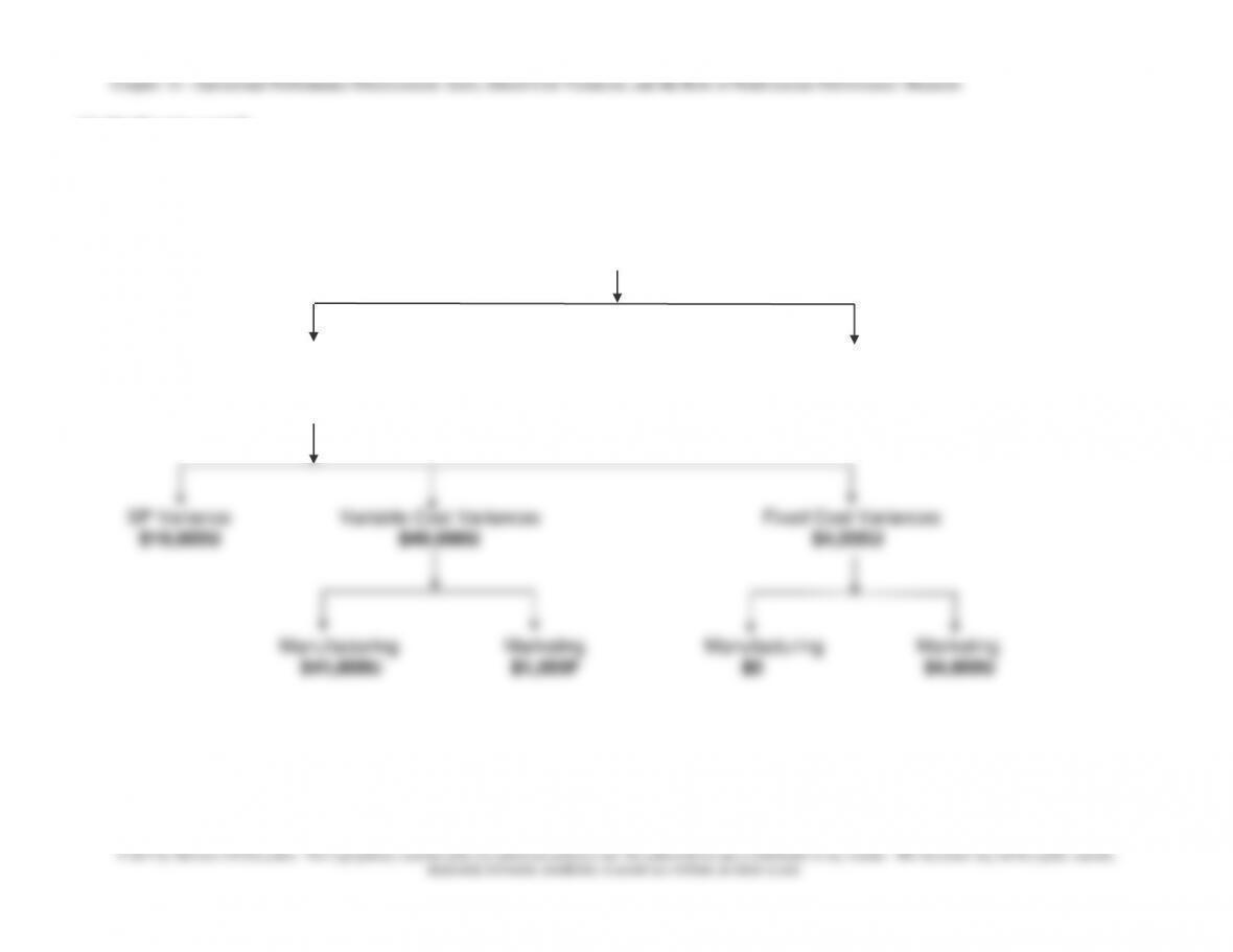
14-43 (Continued-3)
Ortiz & Co.
Master (Static) Budget Variance
(Actual Operating Income − Master Budget Operating Income)
$50,000U
Total FB-Variance Sales Volume Variance
$54,000U $4,000F
($20,000 − $74,000) ($40/unit × 100 units)

Chapter 14 – Operational Performance Measurement: Sales, Direct-Cost Variances, and the Role of Nonfinancial
Performance Measures
14–45
14–43 (Continued-4)
Note to Instructor: An Excel file solution covering parts (1) and (2) of this
assignment is embedded below. You can open this “object” by doing the following:
1. Right click anywhere in the worksheet area below.
2. Select “worksheet object” and then select “Open.”
3. To return to the Word document, select “File” and then “Close and return
to…” while you are in the spreadsheet mode. The screen should then
return you to this Word document.
Solution to Pr. 14-43
(6e).xlsx