Chapter 14 – Operational Performance Measurement: Sales, Direct-Cost Variances, and the Role of Nonfinancial
Performance Measures
14–16
1. Right click anywhere in the worksheet area below.
2. Select “worksheet object” and then select “Open.”
3. To return to the Word document, select “File” and then “Close and return
to…” while you are in the spreadsheet mode. The screen should then
return you to this Word document.
14–27 Master (Static) Budget Variance and Components (45 minutes)
1. Actual operating income = actual sales revenue − actual variable costs − actual
fixed costs = $380,000 − $210,000 − $145,000 = $25,000
2. Master (static) budget operating income = budgeted sales − budgeted variable
costs − budgeted fixed costs = $450,000 − $270,000 − $135,000 = $45,000
3. Total master (static) budget variance, in terms of operating income = actual
b) Sales volume variance, in terms of operating income = flexible-budget
operating income − master budget operating income = $25,000 − $45,000 =
$20,000U.
c) Master budget variance = Total flexible-budget variance + Sales volume
variance = $0 + $20,000U = $20,000U
Solution to Ex. 14-26
(6e).xlsx
Chapter 14 – Operational Performance Measurement: Sales, Direct-Cost Variances, and the Role of Nonfinancial
Performance Measures
14–17
14–27 (Continued)
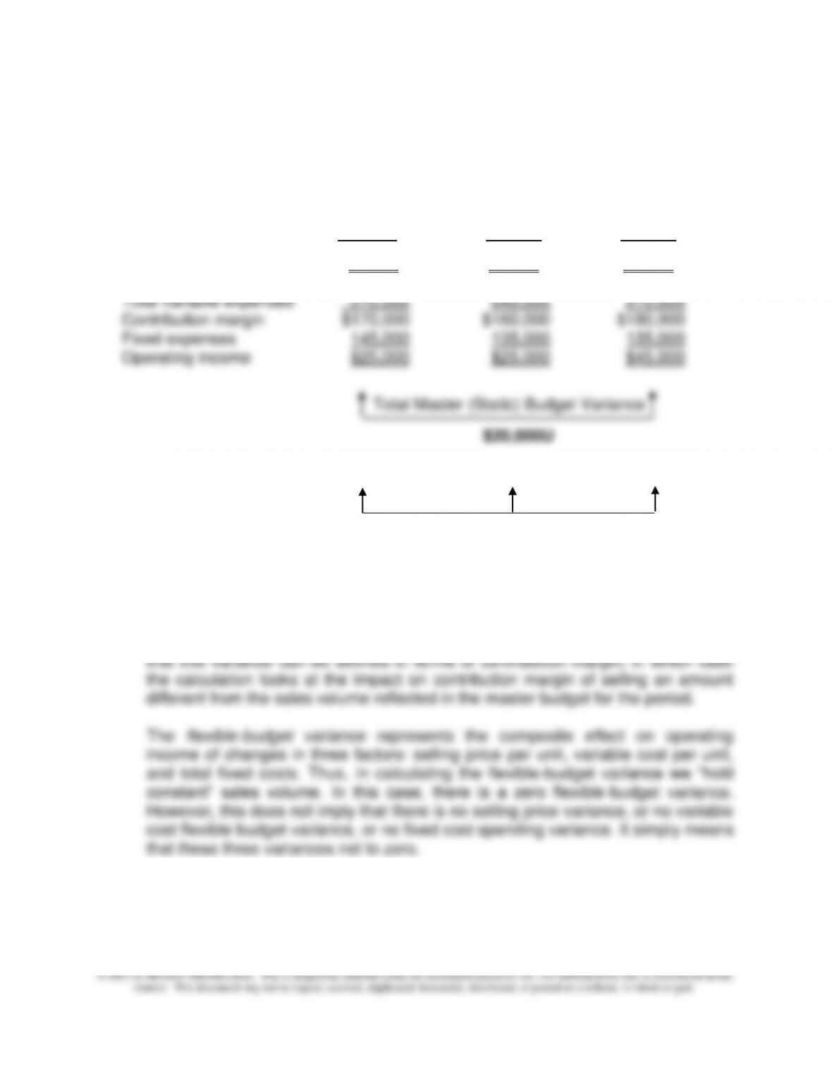
In tabular form, we have:
Actual Flexible Master
Results Budget Budget
Unit sales 40,000 40,000 45,000
Sales $380,000 $400,000 $450,000
Flexible-Budget Sales Volume
Variance Variance
$0 $20,000U
5. The sales volume variance represents the impact on operating profit of selling a
different volume of sales compared to the budgeted volume reflected in the
master budget. As such, the calculation of the variance holds three other factors
constant: selling price per unit, variable cost per unit, and total fixed costs. Note
14–18
© 2013 by McGraw-Hill Education. This is proprietary material solely for authorized instructor use. Not authorized for sale or distribution in any
manner. This document may not be copied, scanned, duplicated, forwarded, distributed, or posted on a website, in whole or part.
14–28 Flexible Budget and Operating-Income Variances (45 minutes)
1. Flexible budget for June, based on 950 units produced/sold (95% of original master
budget):
Units sold 900
Sales (95% × $800,000) $760,000
2. Refer to text Exhibit 14.1 for master-budget data
a. Sales volume variance, in terms of operating income = flexible-budget
operating income – master (static) budget operating income
= $182,500 − $200,000 = $17,500U
b. Sales volume variance, in terms of contribution margin = flexible-budget
contribution margin −master (static) budget contribution margin
3.
Actual Operating Results
For the Month of June
Sales (950 units × $835/unit) $793,250
Less: Total variable expenses 475,000
Chapter 14 – Operational Performance Measurement: Sales, Direct-Cost Variances, and the Role of Nonfinancial
Performance Measures
14–19
14–28 (Continued)
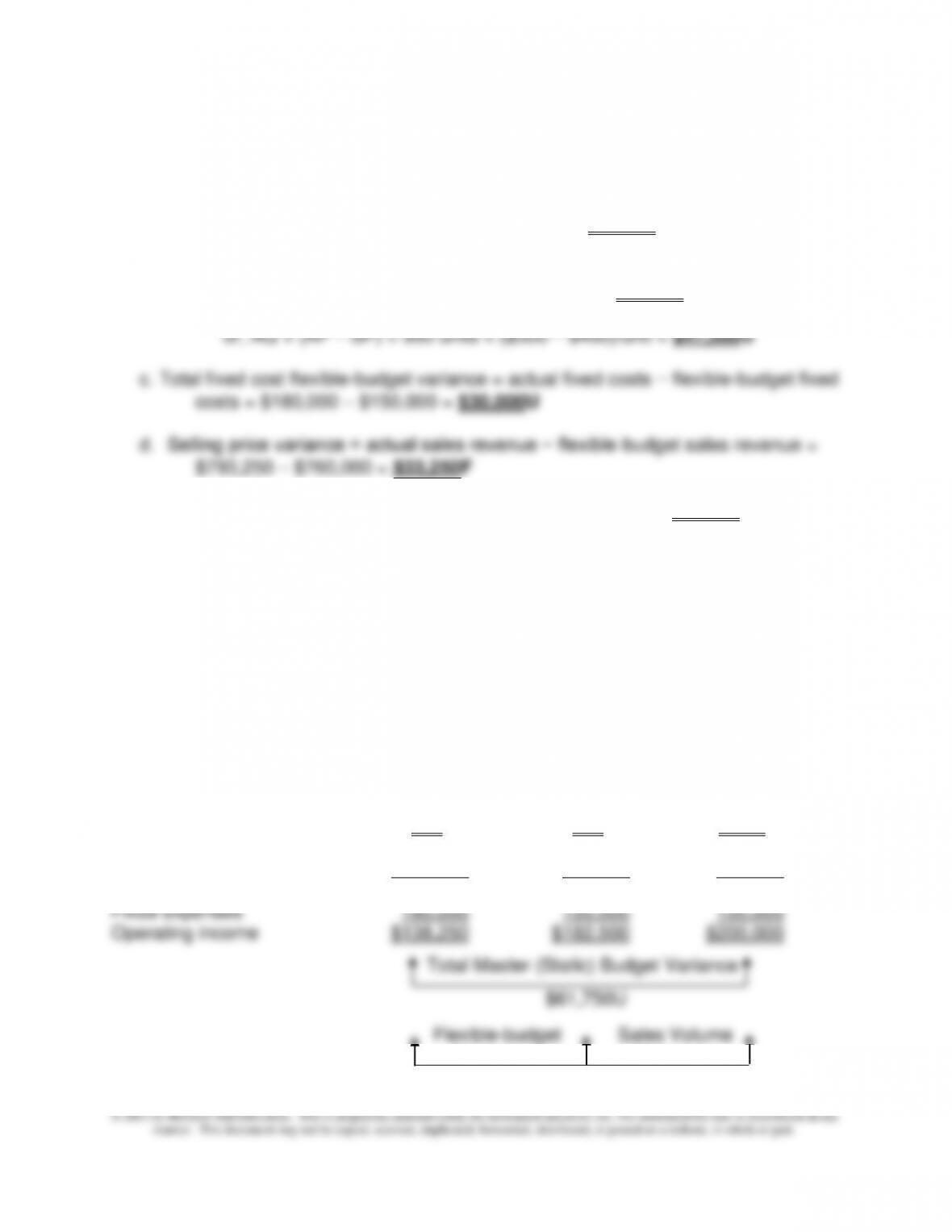
a. Total flexible-budget variance = actual operating income − flexible-budget
operating income = $138,250 − $182,500 = $44,250U
b. Total variable cost flexible-budget variance = actual variable costs − flexible-
budget variable costs = $475,000 − $427,500 = $47,500U
or, AQ × (AP − SP) = 950 units × ($835 − $800) = $33,250F
NOTE: total flexible-budget variance ($44,250U) = selling price variance ($33,250F)
+ total variable cost flexible-budget variance ($47,500U) + total fixed cost flexible-
budget variance ($30,000U).
The following presentation, similar to text Exhibit 14.4, might be useful for in-class
presentation purposes:
SCHMIDT MACHINERY COMPANY
Analysis of Operating Results
June 2013
Flexible Static (Master)
Actual Budget Budget
Unit sales 950 950 1,000
Sales $793,250 $760,000 $800,000
Total variable expenses 475,000 427,500 450,000
Contribution margin $318,250 $332,500 $350,000
Variance Variance
$44,250U $17,500U
Chapter 14 – Operational Performance Measurement: Sales, Direct-Cost Variances, and the Role of Nonfinancial
Performance Measures
14–20
14–29 Direct Materials and Direct Labor Variances (30 minutes)
Note: Refer to Exhibit 14.5 for standard cost information.
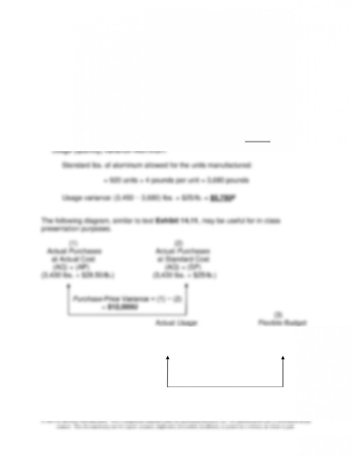
1. Purchase price variance–Aluminum:
Total lbs. aluminum purchased = lbs. used + ending inventory −
beginning inventory = 3,450 + 30 − 50 = 3,430 pounds
Purchase–price variance = ($28.50 − $25)/lb. × 3,430 lbs. = $12,005U
at Standard Cost Amount
(AQ) × (SP) (SQ) × (SP)
(3,450 lbs. × $25/lb.) (3,680 lbs. × $25/lb.)
Usage Variance = (2) − (3)
= $5,750F
Chapter 14 – Operational Performance Measurement: Sales, Direct-Cost Variances, and the Role of Nonfinancial
Performance Measures
14–21
14–29 (Continued)
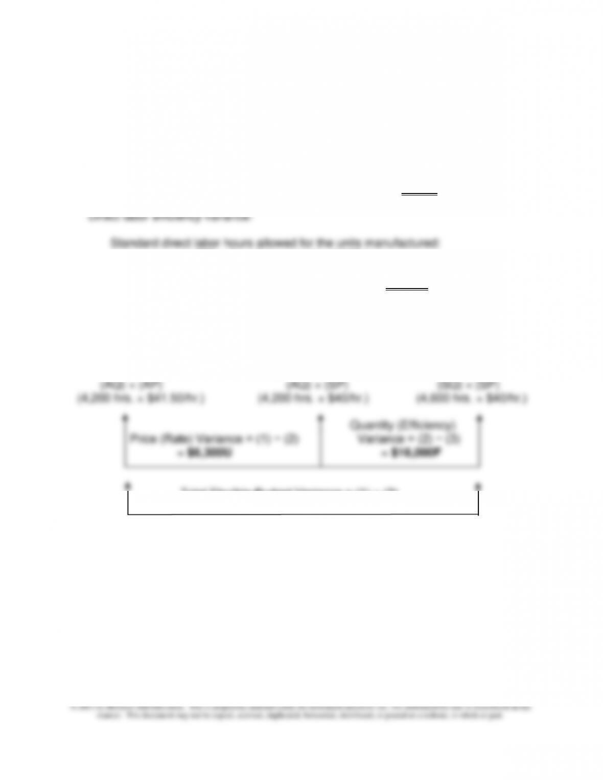
2. Direct labor rate variance: ($41.50 − $40)/hr. × 4,200 hrs. = $6,300U
920 units × 5 hours/unit = 4,600 hours
Efficiency variance: (4,200 − 4,600) hrs. × $40/hr. = $16,000F
The following diagram, similar to text Exhibit 14.7, may be useful for in-class
presentation purposes:
(2) (3)
(1) Actual Input Flexible-budget
Actual Input Cost at Standard Cost Amount
Total Flexible-Budget Variance = (1) − (3)
= $174,300 − $184,000 = $9,700F
14–22
© 2013 by McGraw-Hill Education. This is proprietary material solely for authorized instructor use. Not authorized for sale or distribution in any
manner. This document may not be copied, scanned, duplicated, forwarded, distributed, or posted on a website, in whole or part.
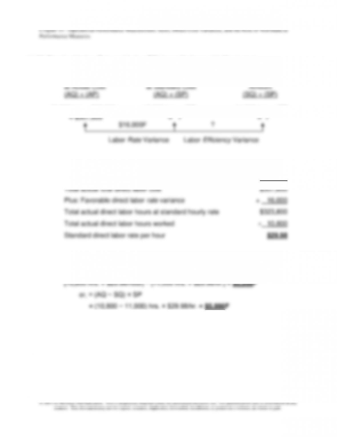
14–30 Standard Labor Rate and Labor Efficiency Variance (15-20 minutes)
Actual Inputs Actual Inputs Flexible-Budget
10,800 hrs. × $28.50/hr. 10,800 hrs. × (SP) 11,000 hrs. × (SP)
1. Total actual direct labor hours worked 10,800
Actual hourly rate × $28.50
2. Direct labor efficiency variance = actual hours at standard cost − standard labor
cost for units produced = [(AQ) × (SP)] − [(SQ) × (SP)] =
14–23
© 2013 by McGraw-Hill Education. This is proprietary material solely for authorized instructor use. Not authorized for sale or distribution in any
manner. This document may not be copied, scanned, duplicated, forwarded, distributed, or posted on a website, in whole or part.
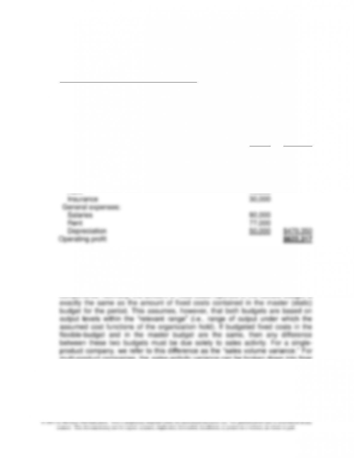
14–31 Generating a Flexible Budget; Spreadsheet Application (45–50 minutes)
1. Flexible Budget, sales volume = 55,000 units
Sales (55,000 units × $31.00/unit) $1,705,000
Less: Cost of Goods Sold:
Direct materials (55,000 units × $2.766666/unit) $152,157
Direct labor (55,000 units × $7.50/unit) 412,500
Manufacturing overhead:
Rent 77,000
Depreciation 50,000 $442,450
Operating profit $472,883
Note to Instructor: An Excel file solution for Part 1 and Part 2 of Exercise 14–31 is
embedded below. You can open this “object” by doing the following:
1. Right click anywhere in the worksheet area below.
2. Select “worksheet object” and then select “Open.”
3. To return to the Word document, select “File” and then “Close and return
to…” while you are in the spreadsheet mode. The screen should then
return you to this Word document.
Ex. 14-31.xlsx
Chapter 14 – Operational Performance Measurement: Sales, Direct-Cost Variances, and the Role of Nonfinancial
Performance Measures
14–24
14–31 (Continued)
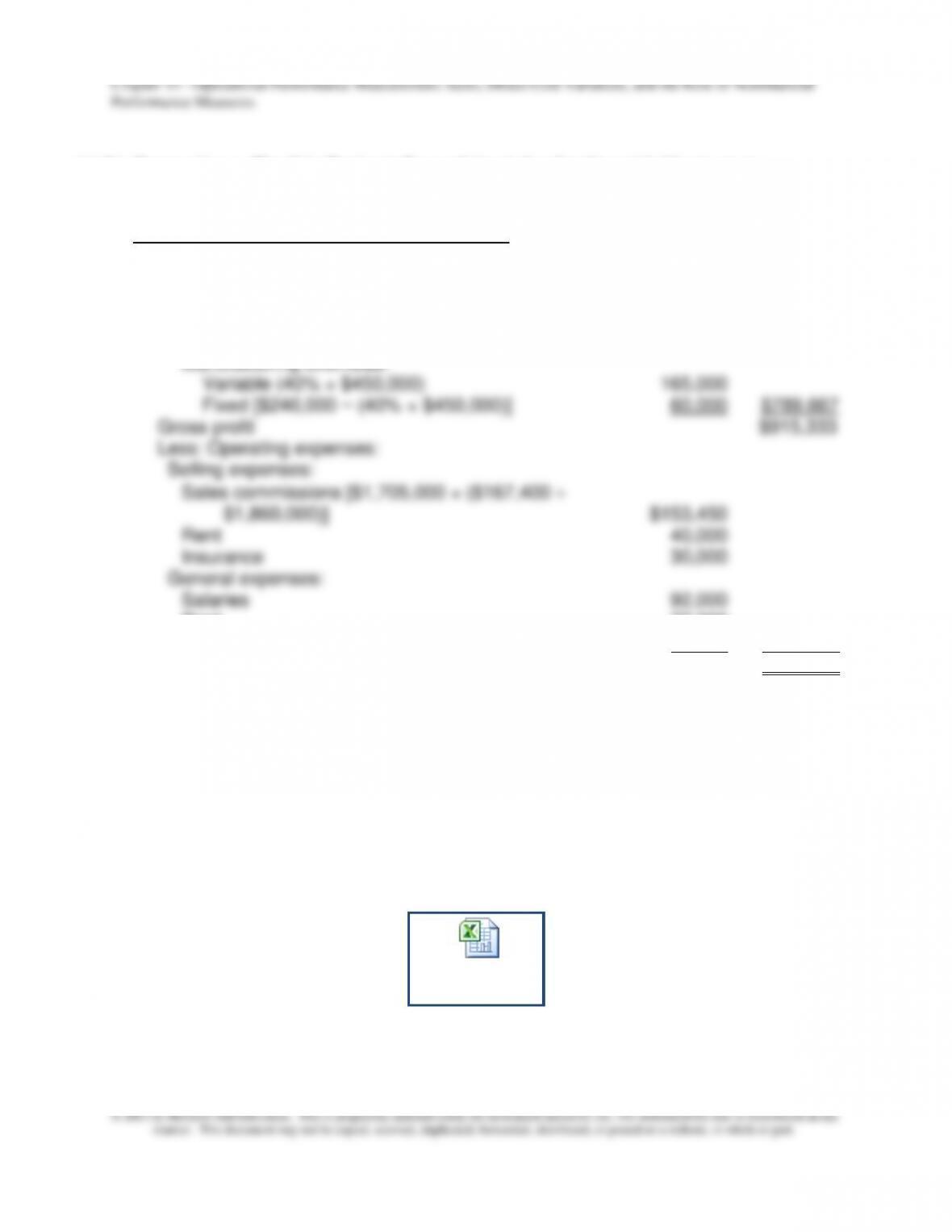
2. Flexible budget, sales volume = 65,000 units
Sales (65,000 units × $31.00/unit) $2,015,000
Less: Cost of Goods Sold:
Direct materials (65,000 units × $2.7666666/unit) $179,833
Direct labor (65,000 units × $7.50/unit) 487,500
Manufacturing overhead:
Variable (40% × $487,500) 195,000
Fixed [see answer, Part 1] 60,000 $922,333
Gross profit $1,092,667
Less: Operating expenses:
Selling expenses:
Sales commissions [$2,015,000 × ($167,400
$1,860,000)] $181,350
Rent 40,000
3. The text uses the term pro-forma budget to refer to a budget prepared for any
level of operating activity for a given period. We reserve the term “flexible–budget”
to refer to the control budget prepared after the period based on the actual activity
level (e.g., sales volume) achieved. The flexible-budget is key to the financial
control process: it allows us to decompose overall variances into more detailed
components. Normally, the amount of fixed costs reported in the flexible-budget is
multi-product companies, the sales-activity variance can be broken down into finer
components, as discussed in Chapter 16.
14–25
© 2013 by McGraw-Hill Education. This is proprietary material solely for authorized instructor use. Not authorized for sale or distribution in any
manner. This document may not be copied, scanned, duplicated, forwarded, distributed, or posted on a website, in whole or part.
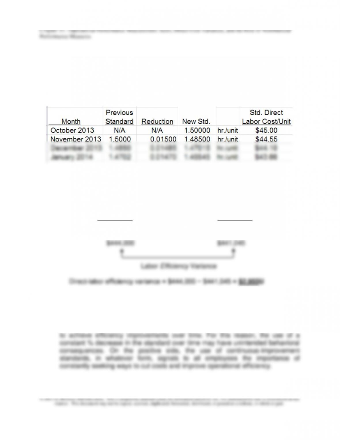
14–32 Behavioral Considerations and Continuous Improvement Standards (20-25
minutes)
1. Direct labor-hour standards and standard direct labor cost per unit, October 2013–
January 2014:
2. Computation of direct labor efficiency variance, December 2013:
Actual Inputs Flexible-Budget
at Standard Cost Amount
(AQ) × (SP) (SQ) × (SP)
14,800 hrs. × $30.00/hr. (10,000 × 1.47015 hrs./unit) × $30.00/hr.
3. The basic trade-off is a problem similar to the situation with Kaizen: pushing
employees too hard for improvements, month after month. In response, workers
may perceive that the performance goal is simply not achievable, in which case
the standard itself loses its motivational value. In many processes, significant
improvements can occur initially. However, it becomes successively more difficult
Chapter 14 – Operational Performance Measurement: Sales, Direct-Cost Variances, and the Role of Nonfinancial
Performance Measures
14–26
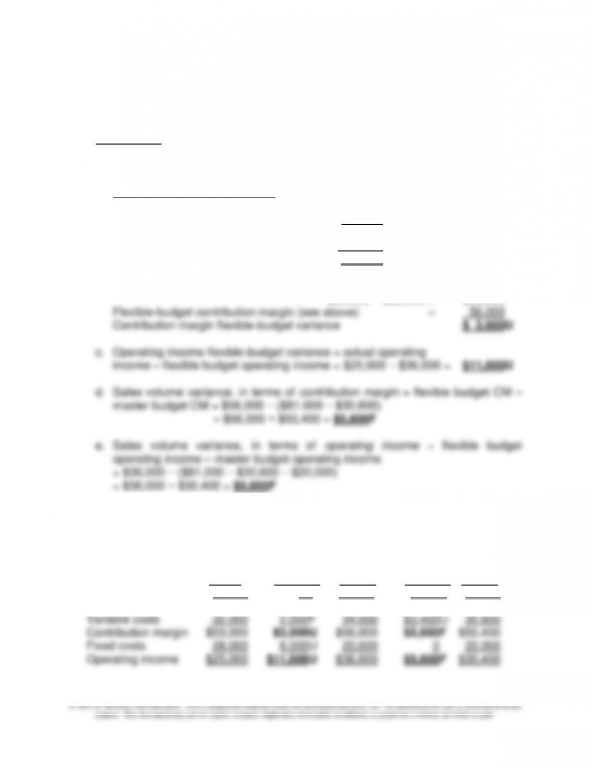
14–33 Flexible Budget and Operating-Income Variances (30-45 minutes)
1. Budget data:
Selling price: $81,000 ÷ 18,000 units = $4.50 per unit
Variable cost : $30,600 ÷ 18,000 units = $1.70 per unit
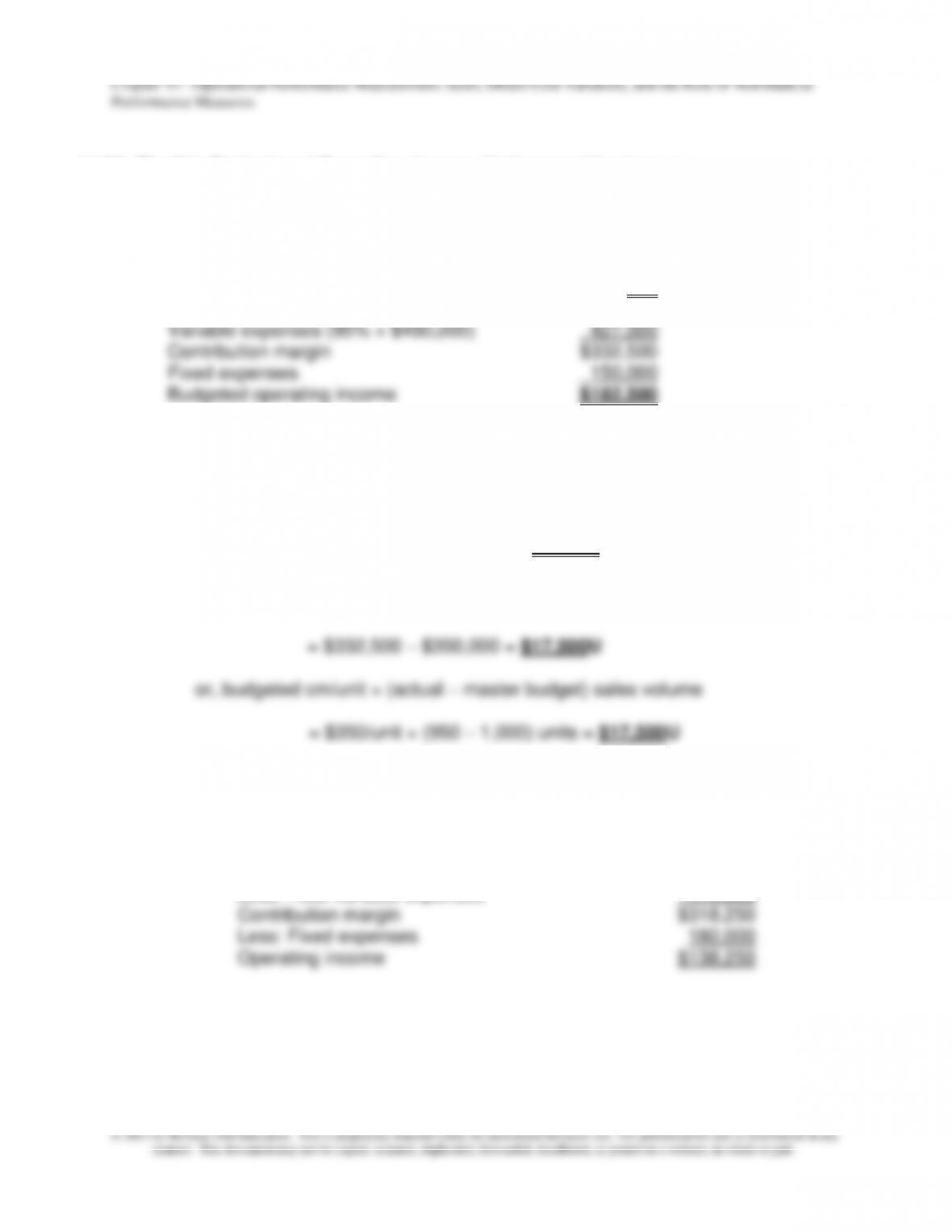
a. Flexible budget for 20,000 units
Sales 20,000 × $4.50 = $90,000
Variable costs 20,000 × $1.70 = 34,000
Contribution margin $56,000
Fixed costs 20,000
Operating income $36,000
b. Contribution margin earned for the period:
$85,000 − $32,000 = $53,000
The following summary, similar to text Exhibit 14.4, may be helpful for in-class
presentation purposes:
Flexible- Sales Master
Budget Flexible Volume (Static)
Actual Variance Budget Variance Budget
Unit sales 20,000 -0- 20,000 2,000F 18,000
Sales $85,000 $5,000U $90,000 $9,000F $81,000
Chapter 14 – Operational Performance Measurement: Sales, Direct-Cost Variances, and the Role of Nonfinancial
Performance Measures
14–27
14–33 (Continued)
2. As long as both the budgeted and the actual operations are within the “relevant
range,” the flexible budget for the actual operating level and the master budget
3. The actual fixed costs for a period are likely to differ from the budgeted amount.
As a result, the contribution margin flexible-budget variance is likely to differ from
the operating income flexible-budget variance. This difference is equal to the total
14–34 Applicability of Standard Cost Systems (30-40 minutes)
1. The major advantages of using a standard cost accounting system include the
following:
▪ Budgeting. Standard costs can be the building blocks for budget preparations
and allow the development of flexible budgets.
▪ Performance evaluation. By comparing actual costs to standard costs, the
only in terms of physical quantities. As another example, standard costs greatly
simplify the operation of a process cost system: the standard costs represent the
costs per equivalent unit (i.e., these costs do not have to be calculated
separately using FIFO or the weighted-average method).
Chapter 14 – Operational Performance Measurement: Sales, Direct-Cost Variances, and the Role of Nonfinancial
Performance Measures
14–28
2. The setting of physical standards such as materials quantities, labor hours, machine
time, and set-up time generally requires information about materials, laborers,
equipment specifications, production procedures, and work flow; this information is
generated from studies conducted by technical personnel and/or from the production
3. a. Because cash-maximization is important for a product classified as a cash cow,
efficiency of operations is essential. Standard costs provide targets for monitoring
costs and identifying inefficiencies so that such problems can be corrected.
Because a cash cow is a slow-growing established product, costs should be fairly
predictable and easy to track.
b. Because a product classified as a question mark is facing strong competition, the
ability to control product costs may be the difference between success and
Chapter 14 – Operational Performance Measurement: Sales, Direct-Cost Variances, and the Role of Nonfinancial
Performance Measures
14–29
14–34 (Continued)
4. In an advanced manufacturing environment, characterized by the increased use of
technology in the manufacturing process and the existence of world-class
competitors, several important criticisms of standard cost systems have been raised
in the literature, including:
▪ The use of such standards, as defined and used conventionally, does not
motivate continuous improvement (Kaizen), which could put the organization at a
competitive disadvantage.
▪ Conventional standard cost systems focus too much on direct labor, which for
▪ Many highly-automated manufacturing processes, based on advanced
manufacturing technologies, are highly reliable and consistent; in this case, the
incremental information to management from standard-cost variances can be
small.
Chapter 14 – Operational Performance Measurement: Sales, Direct-Cost Variances, and the Role of Nonfinancial
Performance Measures
14–30
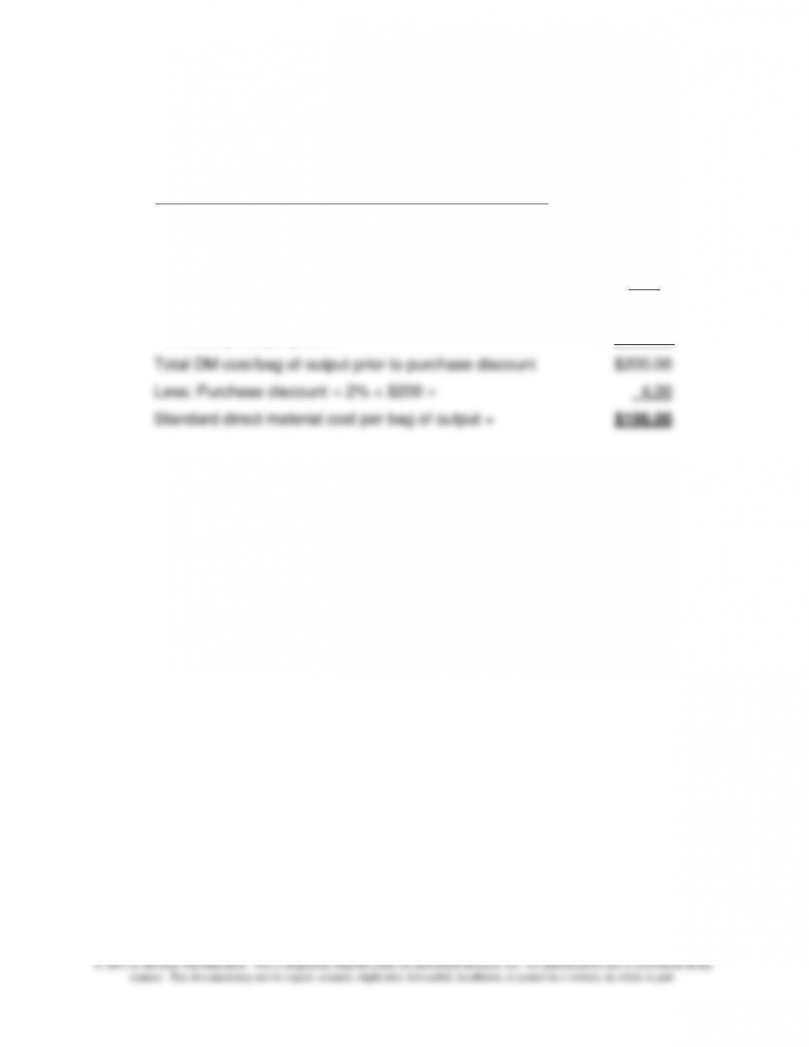
14–35 Determining Standard Direct Materials Cost (10-15 minutes)
Standard direct material cost per bag of Insect-Be-Gone
Total direct materials per unit of output = 60 lbs.
Divided by: Proportion of direct materials inputs remaining
in one unit of finished product = (1 − evaporation rate) = 75%
Total standard quantity of DM inputs/unit of output 80 lbs.
Purchase price per pound × $2.50/lb.