Chapter 12 – Strategy and the Analysis of Capital Investments
12–61
12–50 (Continued-2)
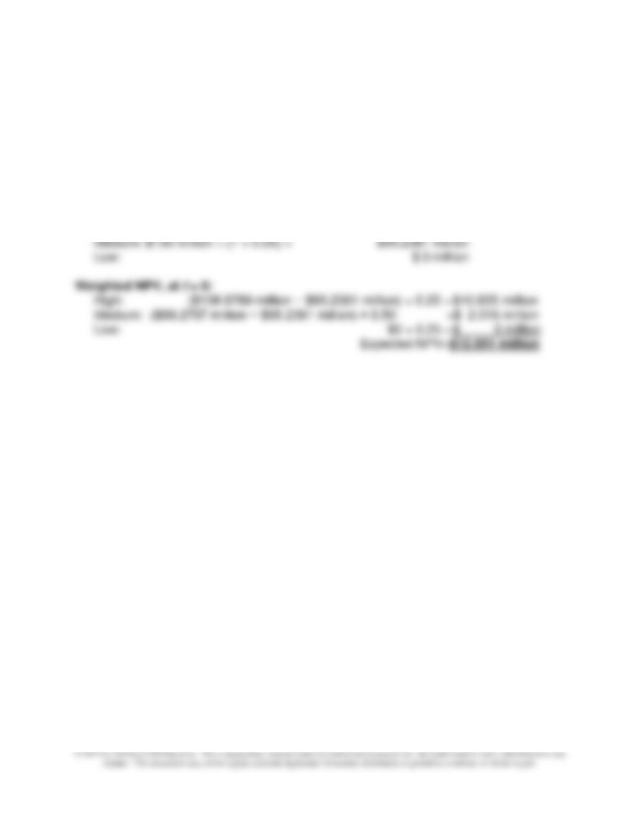
PV of Cash Inflows, at t = 0:
High: (=NPV(0.15,70,70,70)) ÷ (1 + 0.15) = $138.9789 million
Medium: (=NPV(0.15,50,50,50)) ÷ (1 + 0.15) = $99.2707 million
Low: = $0 (do not invest in this situation) $0 million
PV of Cash Outflows, at t = 0:
High: $100 million ÷ (1 + 0.05) = $95.2381 million
Chapter 12 – Strategy and the Analysis of Capital Investments
12–62
12–51 Real Options and Sensitivity Analysis(60 Minutes)
1.
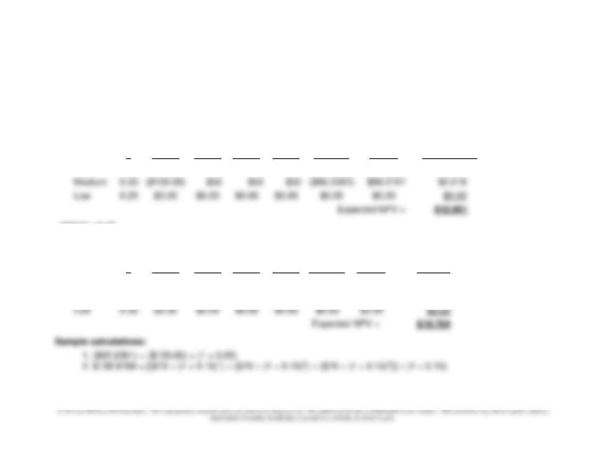
ORIGINAL ASSUMPTION:
WACC =0.15
Risk-Free Rate =0.05
Scenario
p
Year 1
Year 2
Year 3
Year 4
@ t = 0
PV of
Outflows
@ t = 0
PV of
Inflows
Weighted
NPV (@ t =0)
High
0.25
($100.00)
$70
$70
$70
($95.2381)
$138.9789
$10.935
Medium
0.50
($100.00)
$50
$50
$50
($95.2381)
$99.2707
$2.016
Low
0.25
$0.00
$0.00
$0.00
$0.00
$0.00
$0.00
$0.00
Expected NPV =
$12.951
WACC =0.15
Risk-Free Rate = 0.05
Scenario
p
Year 1
Year 2
Year 3
Year 4
@ t = 0
PV of
Outflows
@ t = 0
PV of
Inflows
Weighted NPV
(@ t =0)
High
0.20
($100.00)
$70
$70
$70
($95.24)
$138.98
$8.748
Medium
0.50
($100.00)
$50
$50
$50
($95.24)
$99.27
$2.016
Low
0.30
$0.00
$0.00
$0.00
$0.00
$0.00
$0.00
$0.00
Expected NPV =
$10.764
Sample calculations:
1. ($95.2381) = ($100.00) ÷ (1 + 0.05)
2. $138.9789 = [($70 ÷ (1 + 0.15)1) + ($70 ÷ (1 + 0.15)2) + ($70 ÷ (1 + 0.15)3)] ÷ (1 + 0.15)

Chapter 12 – Strategy and the Analysis of Capital Investments
3. $8.75 = [$138.9789 − $95.2381] × 0.2012–51 (Continued-1)
2. Demand Probabilities: 30%, 40%, 30%
WACC =0.15
Risk-free rate = 0.05
Scenario
p
Year 1
Year 2
Year 3
Year 4
@ t = 0
PV of
Outflows
@ t = 0
PV of
Inflows
Estimated
NPV (@ t =0)
High
0.30
($100.00)
$70
$70
$70
($95.2381)
$138.9789
$13.122
Medium
0.40
($100.00)
$50
$50
$50
($95.2381)
$99.2707
$1.613
Low
0.30
$0.00
$0.00
$0.00
$0.00
$0.00
$0.00
$0.000
Expected NPV =
$14.735
Sample calculations:
1. ($95.2381) = ($100.00) ÷ (1 + 0.05)
2. $138.9789 = ([$70 ÷ (1 + 0.15)1] + [$70 ÷ (1 + 0.15)2] + [$70 ÷ (1 + 0.15)3]) ÷ (1+ 0.15)
3. $13.1223 = [$138.9789 − $95.2381] × 0.30
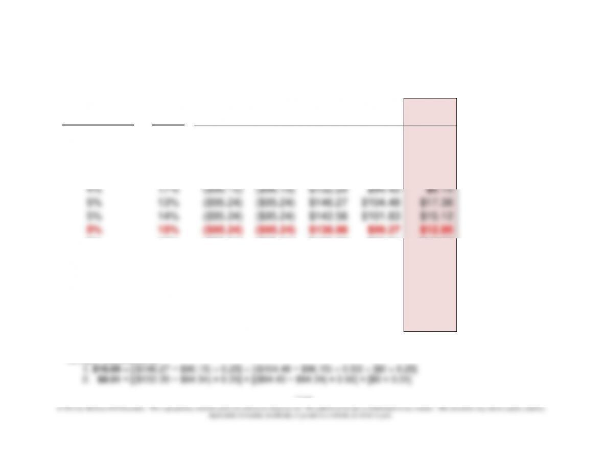
3. Sensitivity Analysis: Assumptions Regarding Discount Rates
@ t = 0
@ t = 0
Weighted
Cash Flows
PV of
PV of
NPV @
Scenario
p
Year 1
Year 2
Year 3
Year 4
Outflows
Inflows
t =0)
High
0.25
($100.00)
$70
$70
$70
($95.2381)
$138.9789
$10.935
Medium
0.50
($100.00)
$50
$50
$50
($95.2381)
$99.2707
$2.016
Low
0.25
$0.00
$0.00
$0.00
$0.00
$0.00
$0.00
$0.00
Expected NPV =
$12.951
Chapter 12 – Strategy and the Analysis of Capital Investments
12–64
12-51 (Continued–2)
PV of Outflows
PV of Inflows
Expected
Risk-Free Rate
WACC
High
Medium
High
Medium
NPV
4%
13%
($96.15)
($96.15)
$146.27
$104.48
$16.69
4%
14%
($96.15)
($96.15)
$142.56
$101.83
$14.44
4%
15%
($96.15)
($96.15)
$138.98
$99.27
$12.26
4%
16%
($96.15)
($96.15)
$135.53
$96.81
$10.17
4%
17%
($96.15)
($96.15)
$132.20
$94.43
$8.15
5%
13%
($95.24)
($95.24)
$146.27
$104.48
$17.38
5%
14%
($95.24)
($95.24)
$142.56
$101.83
$15.12
5%
15%
($95.24)
($95.24)
$138.98
$99.27
$12.95
5%
16%
($95.24)
($95.24)
$135.53
$96.81
$10.86
5%
17%
($95.24)
($95.24)
$132.20
$94.43
$8.83
6%
13%
($94.34)
($94.34)
$146.27
$104.48
$18.05
6%
14%
($94.34)
($94.34)
$142.56
$101.83
$15.80
6%
15%
($94.34)
($94.34)
$138.98
$99.27
$13.63
6%
16%
($94.34)
($94.34)
$135.53
$96.81
$11.53
6%
17%
($94.34)
($94.34)
$132.20
$94.43
$9.51
Sample Calculations:
12–65
12–51 (Continued-3)
Sensitivity Analysis Summary: Estimated NPVs at Time t = 0
Risk-Free Rate
WACC
4%
5%
6%
13%
$16.69
$17.38
$18.05
14%
$14.44
$15.12
$15.80
15%
$12.26
$12.95
$13.63
16%
$10.17
$10.86
$11.53
17%
$8.15
$8.83
$9.51
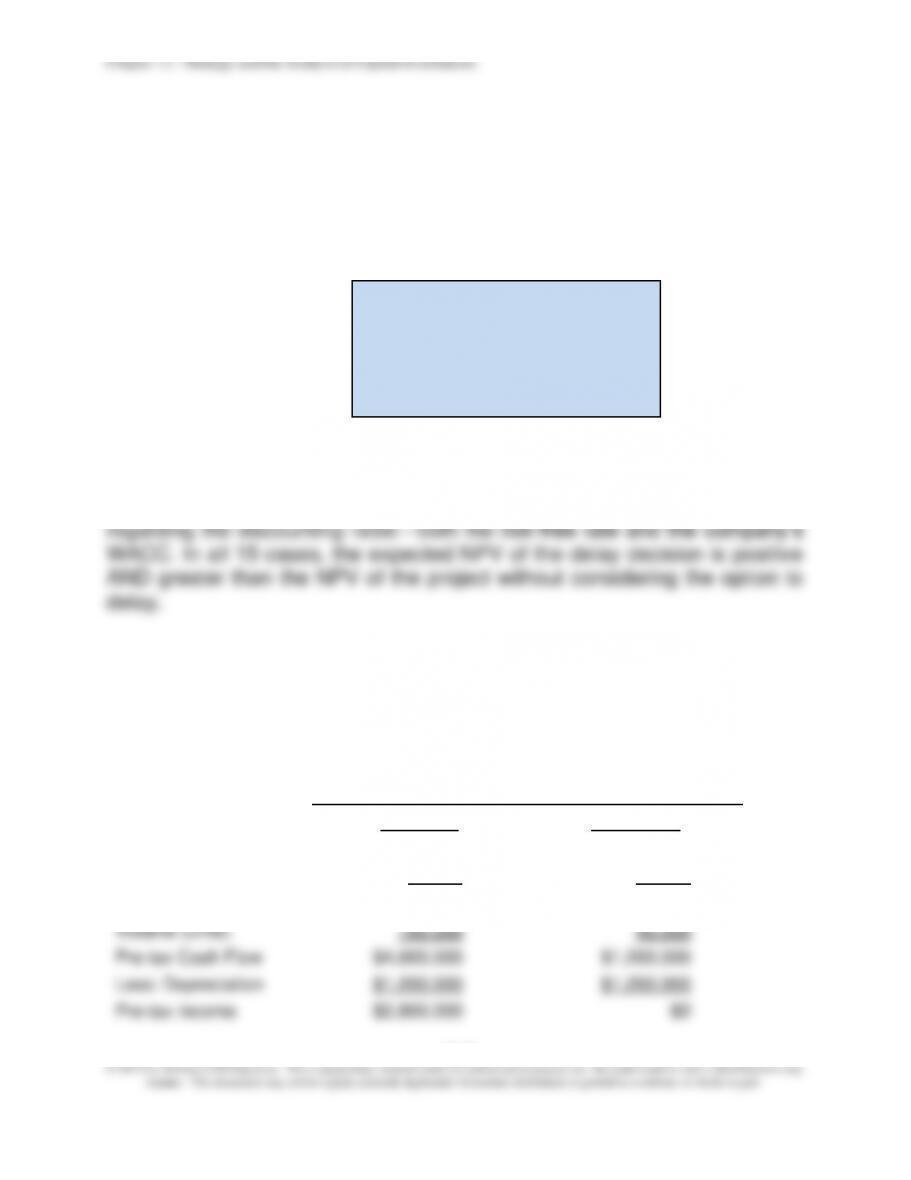
On the basis of the above summary results, we can conclude that the
decision to delay the project one year (to gain better information regarding
the level of consumer demand) is relatively insensitive to assumptions
12–52 Real Options (60 Minutes)
1. Annual after-tax cash flows, both scenarios (possible outcomes):
Product Demand
Optimistic
Pessimistic
Selling price/unit
$80.00
$70.00
Variable cost/unit
$40.00
$40.00
CM/unit
$40.00
$30.00
Volume (units)
100,000
40,000
Pre-tax Cash Flow
$4,000,000
$1,200,000
Less: Depreciation
$1,200,000
$1,200,000
Pre-tax Income
$2,800,000
$0
Chapter 12 – Strategy and the Analysis of Capital Investments
12–66
Taxes
$933,333
$0
After-tax Income
$1,866,667
$0
Plus: Depreciation
$1,200,000
$1,200,000
Net Cash Inflow
$3,066,667
$1,200,000
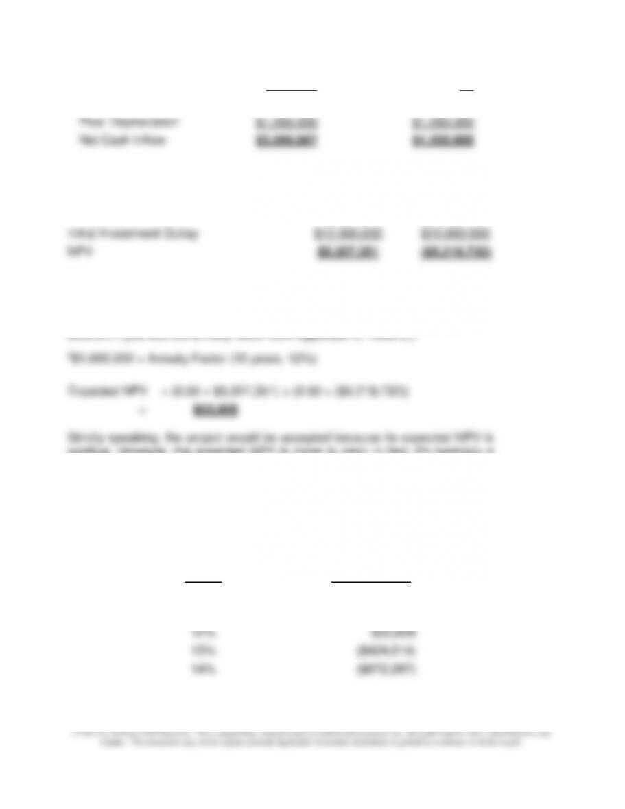
2. Expected NPV of Proposed Investment:
PV of Cash Inflows
$17,327,3511
$6,780,2682
Initial Investment Outlay
$12,000,000
$12,000,000
NPV
$5,327,351
($5,219,732)
Calculations:
1$3,066,667 × Annuity Factor (10 years, 12%) (NOTE: Above answer was
obtained using built-in Excel function, “NPV,” and therefore will be slightly
different if you use the annuity factor from Appendix C, Table 2.)
2$1,600,000 × Annuity Factor (10 years, 12%)
Expected NPV = (0.50 × $5,327,351) + (0.50 × ($5,219,732))
=
$53,809
Strictly speaking, the project would be accepted because its expected NPV is
positive. However, the expected NPV is close to zero; in fact, it’s basically a
“toss up” as to whether or not this project is profitable in a present-value
sense.
12–52 (Continued)
3. Sensitivity Analysis Results:
WACC
Expected NPV
10%
$1,108,410
11%
$563,695
12%
$53,809
13%
($424,014)
14%
($872,287)
Chapter 12 – Strategy and the Analysis of Capital Investments
12–67
Sample Calculation:
$1,108,410 = ([PV of Optimistic Cash Inflows × Annuity Factor, 10 years, 10% × 0.50] +
[PV of Pessimistic Cash Inflows × Annuity Factor, 10 years, 10%]) − $12,000,000
Note: the figures reported above were generated in Excel, using the built-in NPV
function. Because the annuity factors in Table 2 are rounded (to three decimal places),
your answers will be slightly different from the above if you use the annuity factors
rather than the built-in Excel function.
As can be seen from the above results, the Expected NPV (given the indicated
probabilities for each outcome/state-of-nature) is sensitive to the assumption regarding
the discount rate.
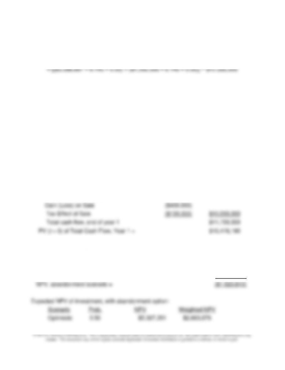
4. Inclusion of abandonment option:
Abandonment value, end of year 1
$10,400,000
Cash flow, end of year 1:
After-tax operating cash flow
$1,200,000
Gross proceeds, equipment
$10,400,000
Less: NBV, end of year 1
$10,800,000
Gain (Loss) on Sale
($400,000)
Tax Effect of Sale
($133,333)
$10,533,333
Total cash flow, end of year 1
$11,733,333
PV (t = 0) of Total Cash Flow, Year 1 =
$10,476,190
12–52 (Continued-2)
NPV of project, with abandonment option:
PV of Total Cash Flow, Year 1
$10,476,190
Less: Investment Outlay, t = 0
$12,000,000
NPV, abandonment scenario =
($1,523,810)
Expected NPV of investment, with abandonment option:
Scenario
Prob.
NPV
Weighted NPV
Optimistic
0.50
$5,327,351
$2,663,676
Chapter 12 – Strategy and the Analysis of Capital Investments
12–68
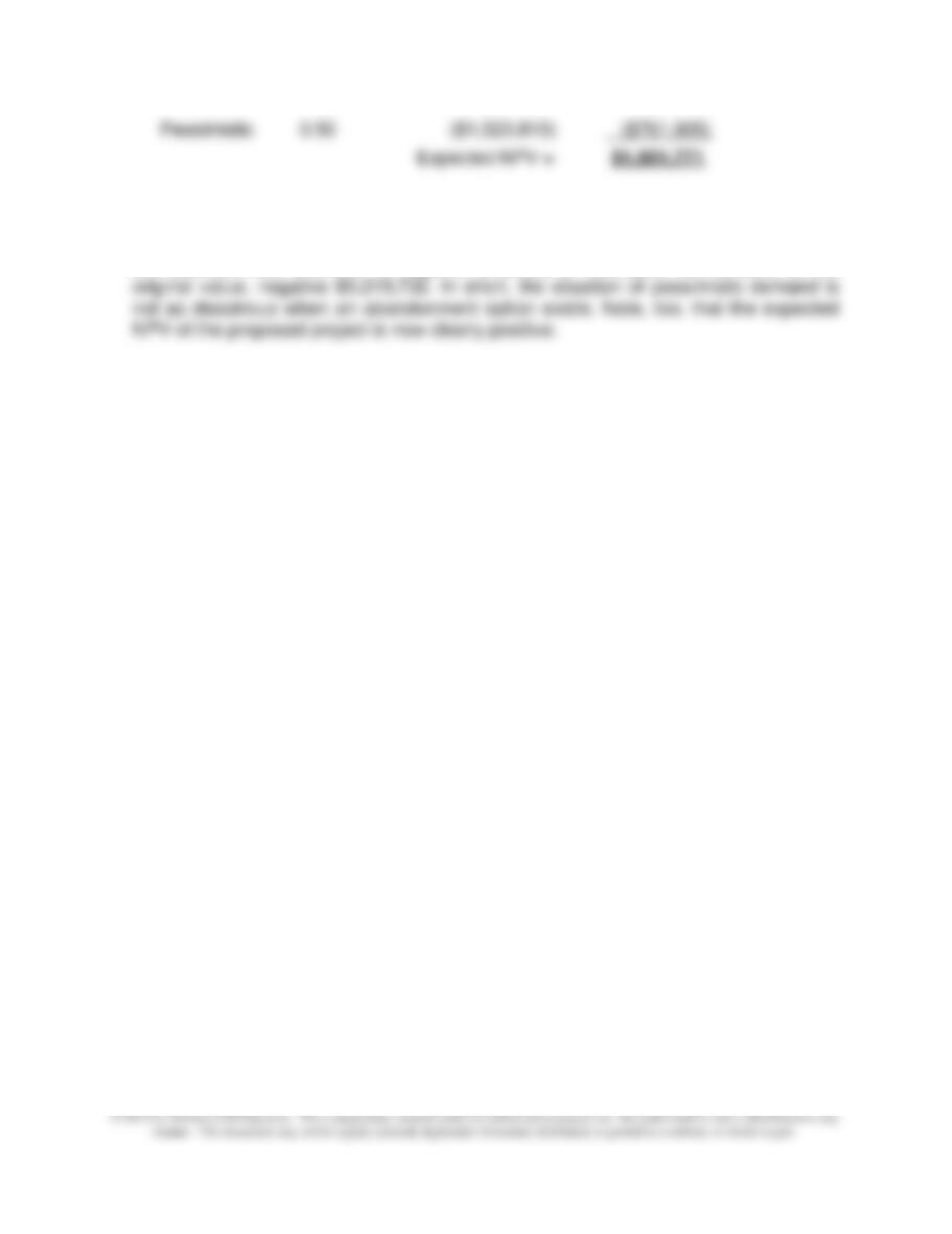
Pessimistic
0.50
($1,523,810)
($761,905)
Expected NPV =
$1,901,771
Note that the abandonment option adds considerable value to the proposed
investment: if demand turns out to be “pessimistic,” then the company can minimize
its losses by abandoning the project at the end of year 1. As you can see, the NPV in
the abandonment scenario is negative $1,523,810. Compare this amount to the
12–69
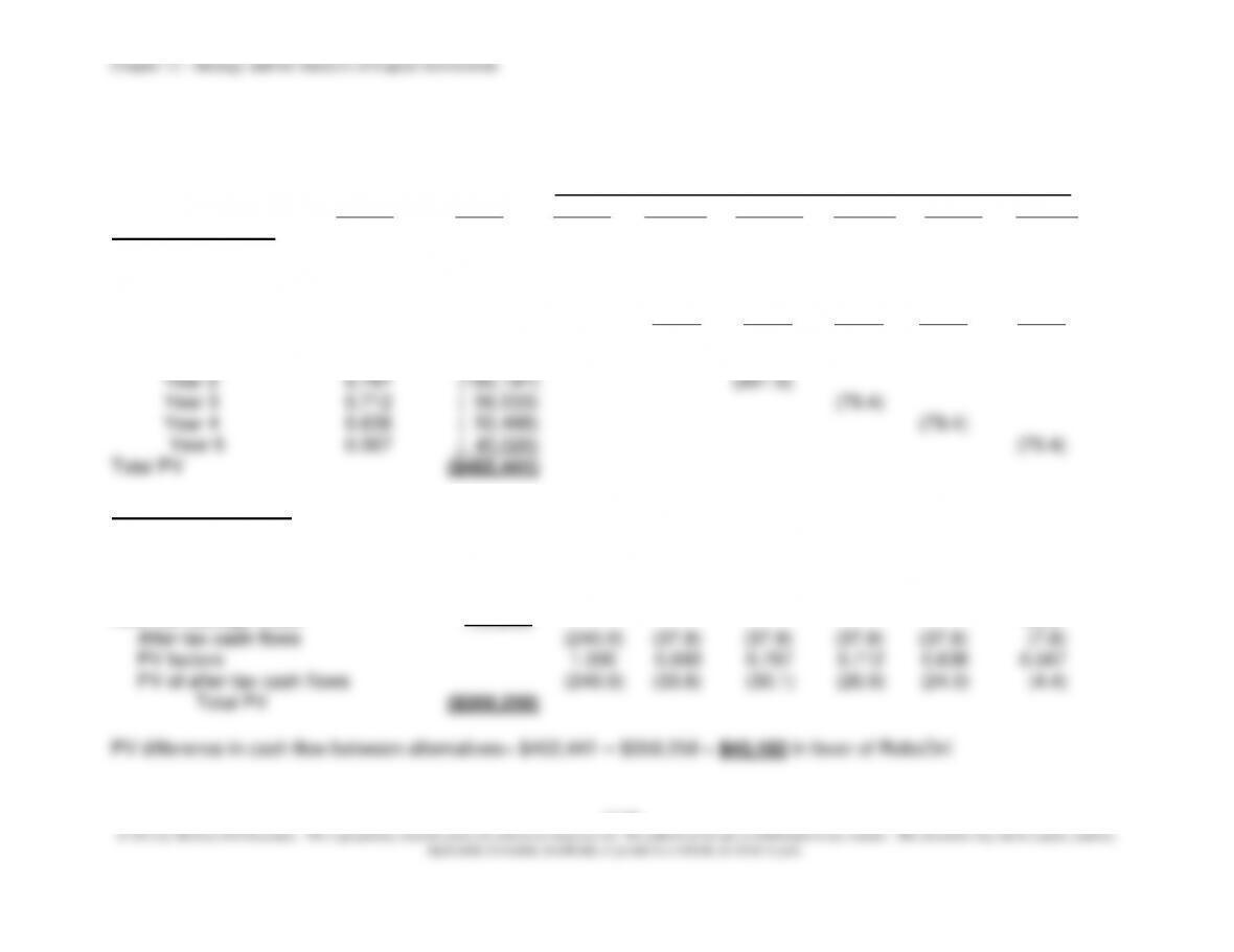
12–53 Equipment-Replacement Decision; Strategy (60 min)
1. & 3.
PV Present After-tax Cash Flows (000s)
Factor Value 0 1 2 3 4 5
Overhaul AccuDril
Operating Cost1 (48.0) (48.0) (38.4) (38.4) (38.4)
Overhaul cost (capitalized) (100.0)
Tax savings on deprec.2 4.0 4.0 16.0 16.0 16.0
Other cash expenses, after tax3 (57.0) (57.0) (57.0) (57.0) (57.0)
After-tax cash flows:
Year 1 0.893 ($90,193) (101.0)
Buy RoboDril 1010K
Net Equip. Purchase4 ($240,000) (240.0)
After-tax cash operating costs5 (86,520) (24.0) (24.0) (24.0) (24.0) (24.0)
Tax savings on depr.6 69,216 19.2 19.2 19.2 19.2 19.2
Other cash expenses, after tax7 (118,965) (33.0) (33.0) (33.0) (33.0) (33.0)
After-tax salvage value8 17,010 30.0
12–70
12–53(Continued–1)
NOTES
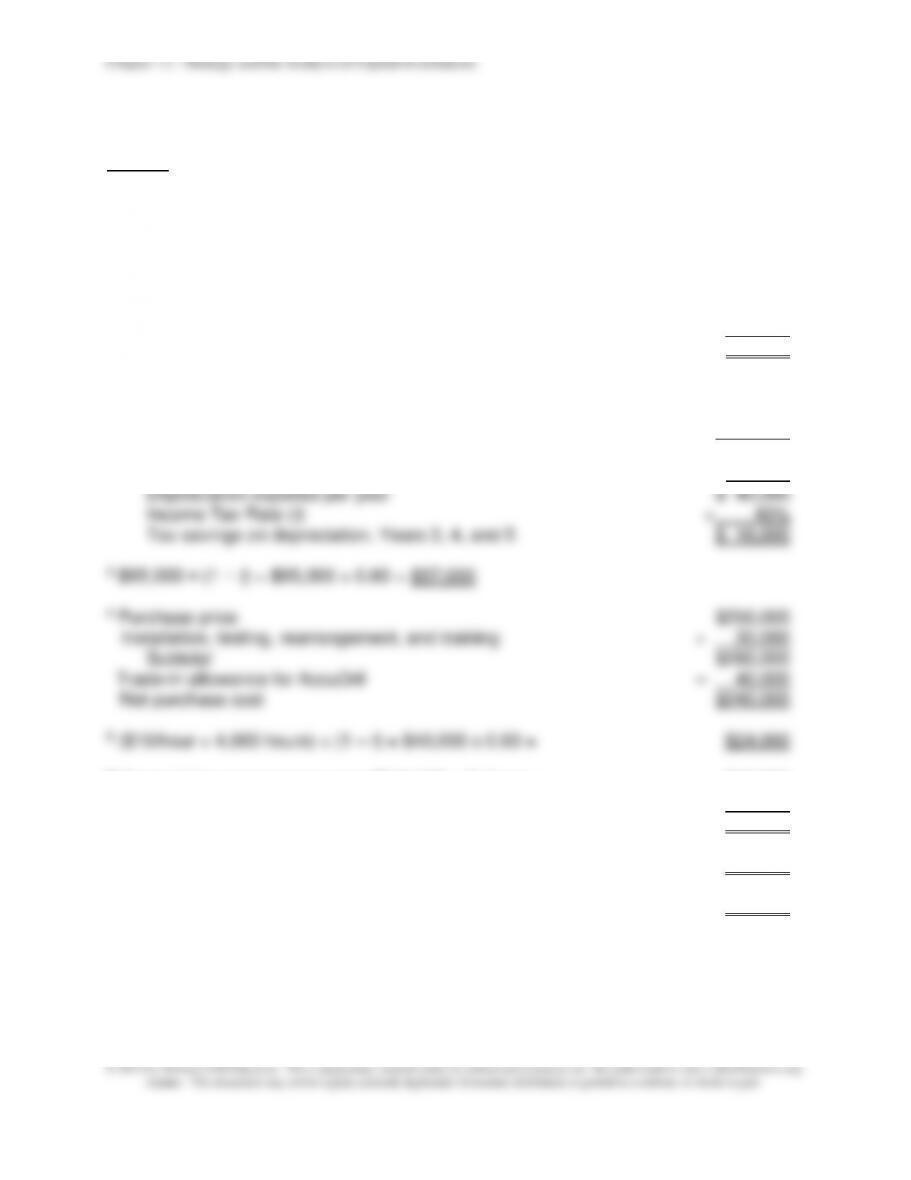
1Years 1 and 2: $10 per hour × 8,000 hours × (1 − t) = $48,000
Years 3, 4, and 5: $48,000 × (1 − 20%) = $38,400
2Years 1 and 2:
Depreciation expense per year (SL basis):
($120,000 − $20,000) 10 = $10,000
Income Tax Rate (t) × 0.40
Tax savings on depreciation, Years 1 and 2 $ 4,000
Years 3, 4, and 5:
Book value before overhaul (end of original useful life) $ 20,000
Overhaul cost, Year 3 100,000
Total amount to be depreciated $120,000
Number of years 3
6 Depreciation expense per year: $240,000 5 Years = $48,000
Income Tax Rate (t) × 0.40
Annual Tax savings on depreciation deduction $19,200
7 $55,000 × (1 – t) = $55,000 × 0.60 = $33,000
8 ($50,000 – $0) × (1 – t) = $50,000 × 0.60 = $30,000
Chapter 12 – Strategy and the Analysis of Capital Investments
12–71
12–53(Continued-2)
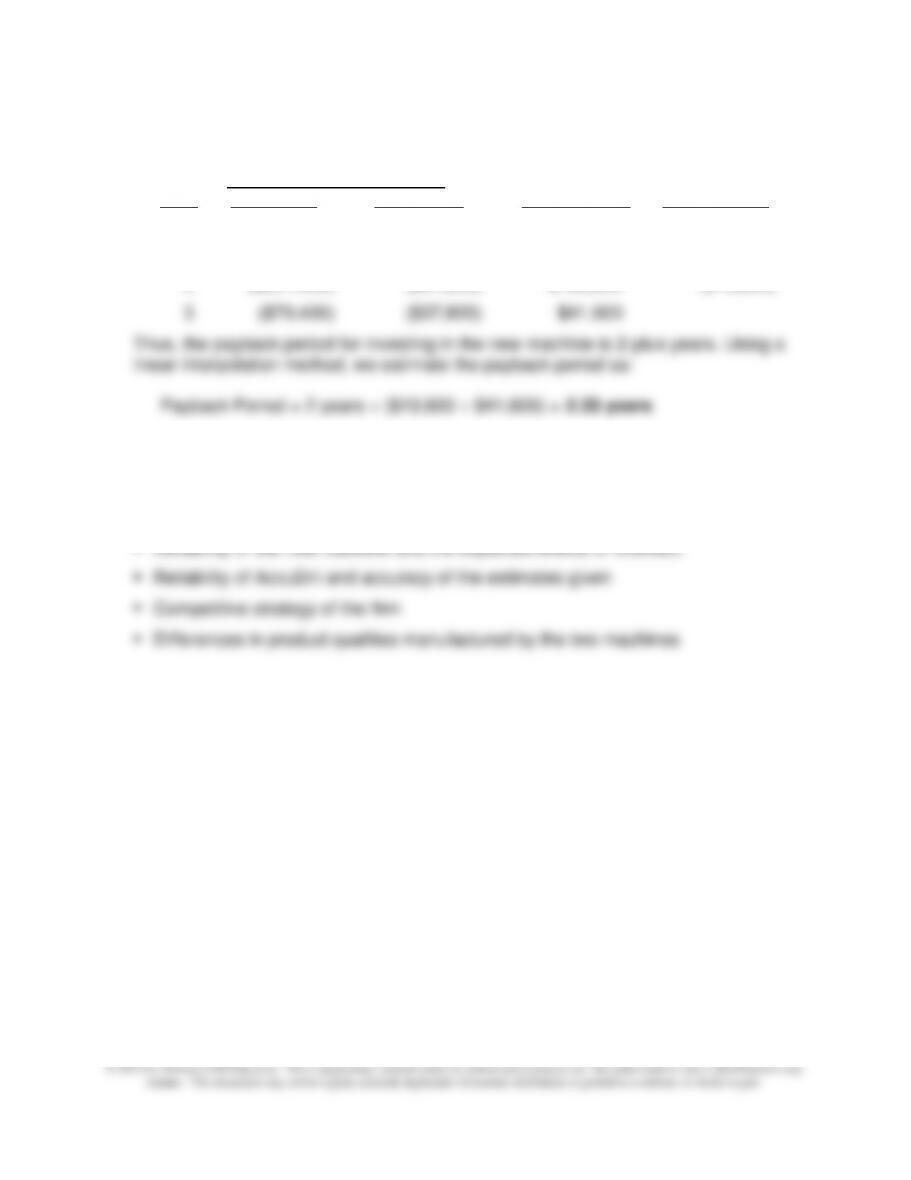
2. Net After-tax Cash Flows Difference in Cumulative
Year AccuDril RoboDril Cash Flows Difference
0 $0 ($240,000) ($240,000) ($240,000)
1 ($101,000) ($37,800) $63,200 ($176,800)
2 ($201,000) ($37,800) $163,200 ($13,600)
4. Among other factors that the firm should consider before the final decision are:
▪ Changes in technology for equipment
▪ Changes in market, especially demand for the product and competitors
▪ Reliability of the new machine and the expected effects of overhaul
12–72
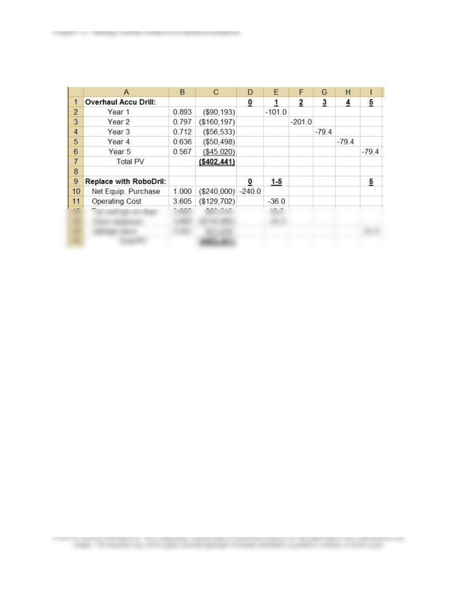
12-54 Sensitivity Analysis; Spreadsheets (75 minutes)
1. Difference in PV between the two alternatives = $402,441 – $359,259 =
$43,182. We focus on the reduction in variable operating cost needed
each year (3 through 5) after the old machine is overhauled.
The equivalent annuity factor needed to convert this stream of after-tax
cash flows (cost savings) to a present value is found in either of two
ways:
(1) Annuity factor (@12%) for three years = 2.402; this annuity factor
needs to be brought back two years, to get a present value of the
Thus, the additional annual after-tax operating cost savings needed from
improvement to make the overhaul of AccuDril a financially attractive
choice = $22,561, as follows:
$43,182 ÷ 1.914 = $22,561
On a before-tax basis (given an income tax rate of 40%), the required
47%.
12–73
12–54 (Continued–1)
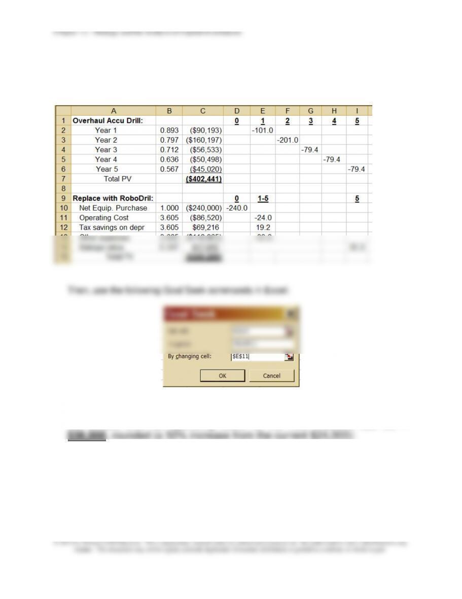
2. The beginning spreadsheet contains the PV of each alternative:
This produces the following result (cell E11): the maximum amount that
the annual after-tax operating costs for the new machine can be =
12–74
12–54 (Continued–2)
Chapter 12 – Strategy and the Analysis of Capital Investments
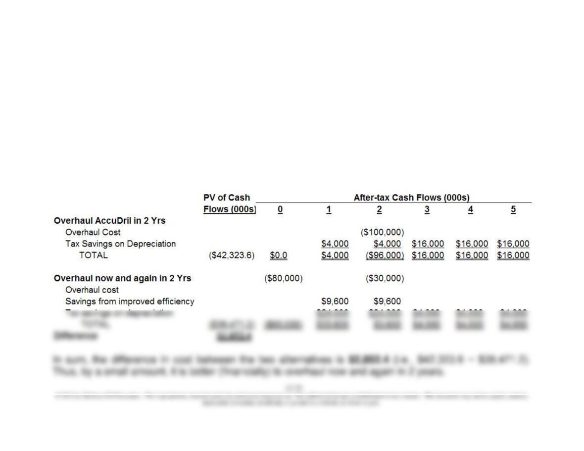
12–54 (Continued-3)
3. Alternative facts:
Revised overhaul cost =
$80,000
Life after first overhaul (in years) =
2
Revised overhaul cost, 2 years hence
$30,000
Life after second overhaul (in years) =
3
Note: the PV cash-flow amounts listed below (viz., ($42,323.6) and ($39,471.2)) were generated using
the NPV built-in function in Excel