Chapter 12 – Strategy and the Analysis of Capital Investments
12–46
12-46 (Continued)
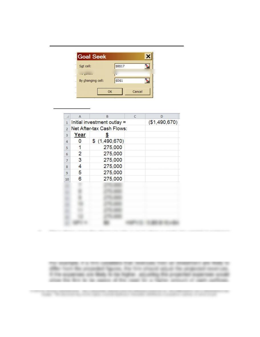
Step 2: Complete the following “Goal Seek” dialog box:
Step 3: Results
4. Many firms raise the discount rate in evaluating a particular capital investment
in view of uncertainties underlying the investment. This approach allows
managers to factor in risks and uncertainties. The higher the risk or uncertainty
a project has, the higher the discount rate.
An alternative is to use a direct approach in dealing with risk or uncertainty.
Chapter 12 – Strategy and the Analysis of Capital Investments
12–47
© 2013 by McGraw-Hill Education. This is proprietary material solely for authorized instructor use. Not authorized for sale or distribution in any
manner. This document may not be copied, scanned, duplicated, forwarded, distributed, or posted on a website, in whole or part.
Some believe that using a direct approach (if possible) is better than simply
using a higher discount rate. In any case, the topic of risk adjustments is
handled more completely in financial management textbooks.
PROBLEMS
12–47 Basic Capital-Budgeting Techniques; No Taxes; Uniform Net Cash Inflows;
Spreadsheets (45-60 minutes)

Chapter 12 – Strategy and the Analysis of Capital Investments
12–48
1. Unadjusted Payback Period: As shown above, the payback period occurs
2. Book (accounting) rate of return (ARR):
As indicated above, the average increase in net income over the ten-year period
= $700,000 ÷ 10 years = $70,000 ÷ year. Thus, the ARR
(a) On initial investment: $70,000 ÷ $500,000 = 14.00%
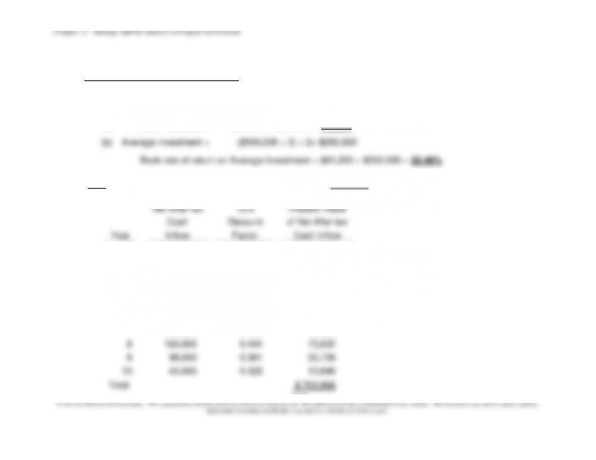
(b) On average investment:
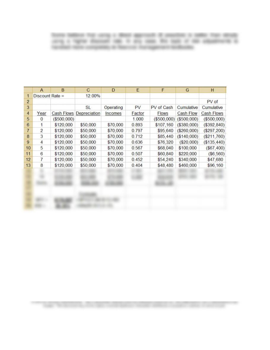
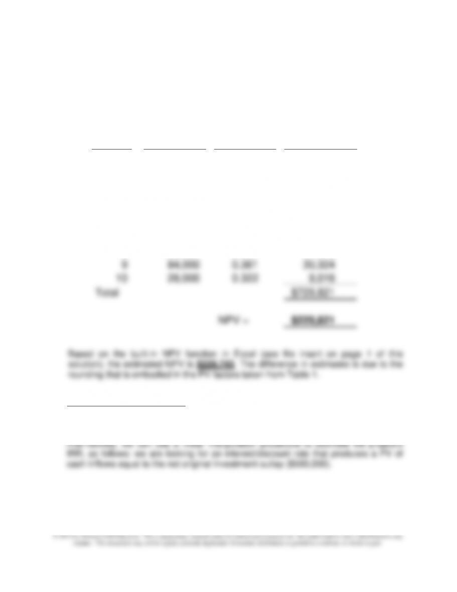
3. NPV: using the PV factors from Appendix C, Table 2, NPV =$178,120
Based on the NPV function of Excel, the NPV = $178,027(the difference in NPV
estimates is due to rounding that takes place when using the PV factors
provided in the Table 2 rather than the built-in NPV function)
4. Present value payback period: as indicated in the above schedule, the present
value payback period is “6–plus” years; this is the time it takes for the present
value of future cash inflows to cover the original investment outlay of $500,000.
If we assume that the cash inflows occur evenly throughout the year, then the
payback period for the proposed investment is:
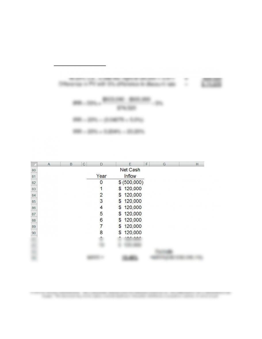
5. Internal rate of return: as indicated in the above schedule, we can use the built–
in function in Excel to estimate the IRR for this proposed investment; IRR =
Chapter 12 – Strategy and the Analysis of Capital Investments
Alternatively, we can estimate the IRR as follows. We are looking for an
interest/discount rate that provides for a NPV = $0 (i.e., a rate that provides a
present value of future cash inflows equal in amount to the original investment
outlay, $500,000). Thus,
PV of net cash inflows:
At 20% (i.e., a rate too low): $120,000 × 4.192 = $503,040
6. Modified internal rate of return (MIRR)—see next page:
12–48 Basic Capital-Budgeting Techniques; Uneven Net Cash Inflows with Taxes and MACRS; Spreadsheet
Application (60-75 minutes)
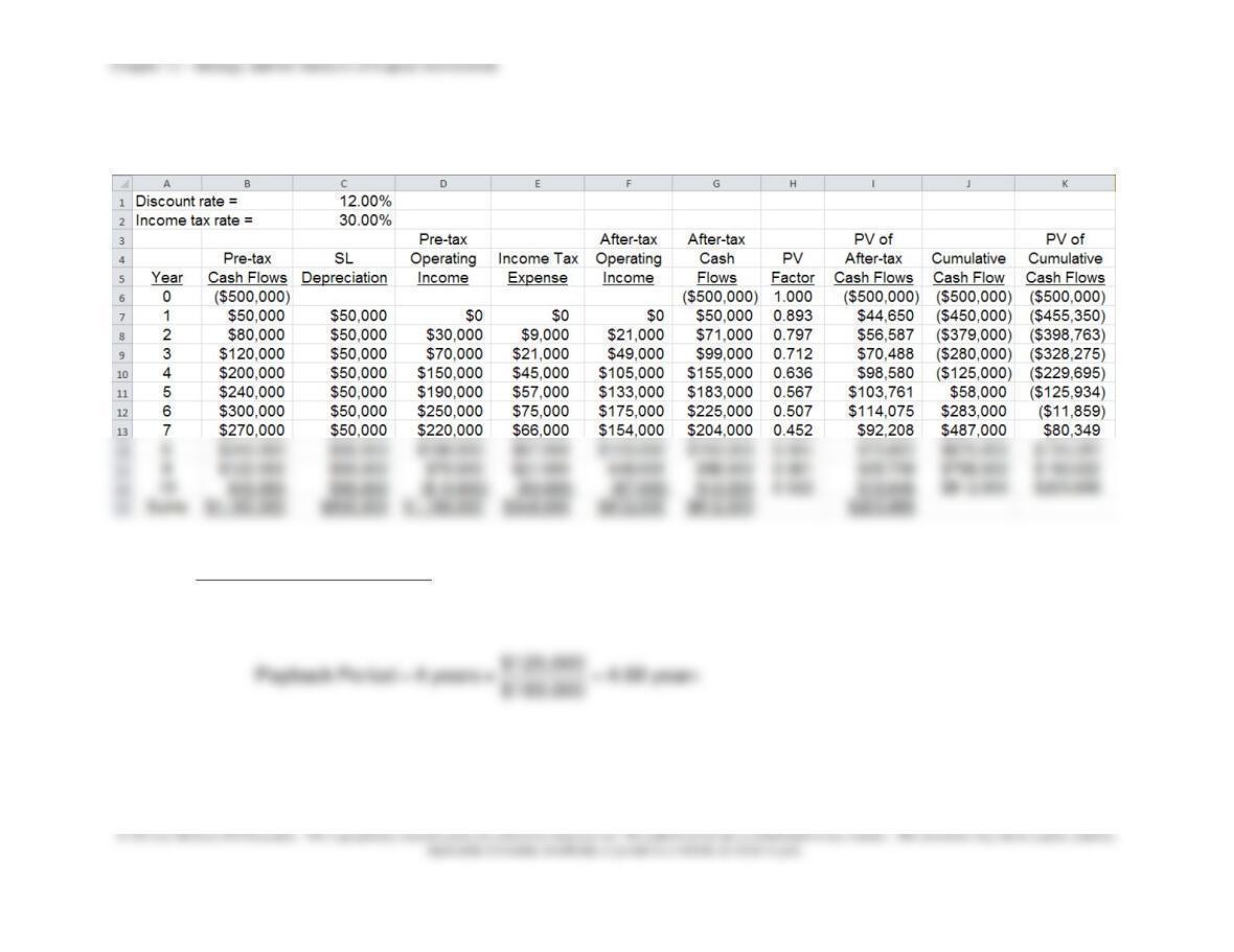
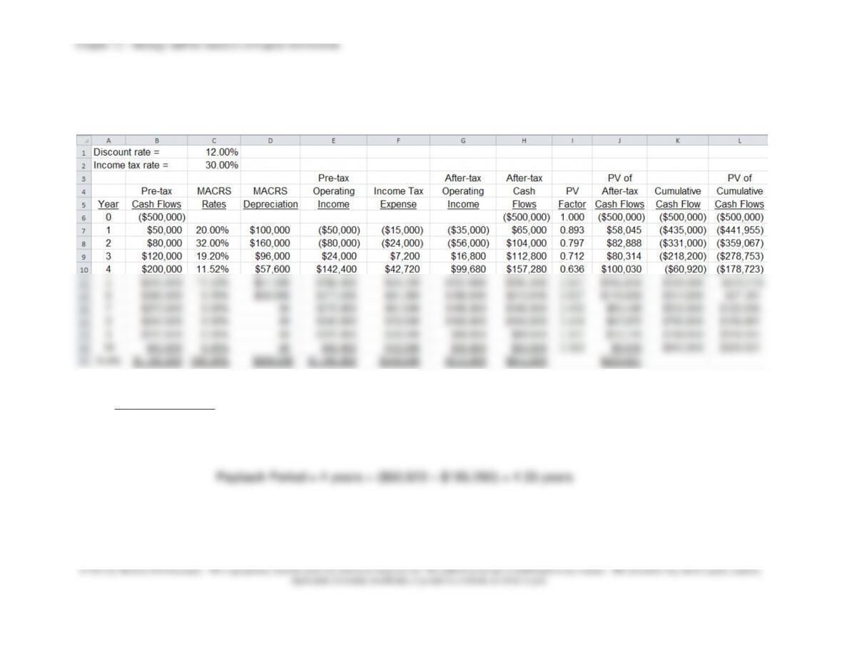
1. Unadjusted Payback Period: as shown by the above schedule, the payback period is between 4 and 5 years.
Under the assumption that the cash inflows occur evenly throughout the year, and using a linear interpolation,
we estimate the payback period as:
12–51
12–48 (Continued-1)
2. Book (accounting) rate of return (ARR):
As indicated above, the average increase in after-tax operating income over the ten-year period = $812,000 ÷ 10
years = $81,200/year. Thus, the ARR
(a) On initial investment: $81,200 ÷ $500,000 = 16.24%
3. NPV: using the PV factors from Appendix C, Table 2, NPV = $203,866
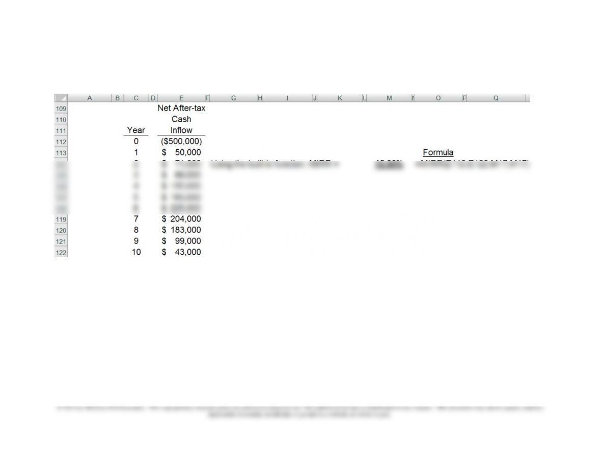
Net After-tax
12%
Present Value
Cash
Discount
of Net After-tax
Year
Inflow
Factor
Cash Inflow
1
$ 50,000
0.893
$ 44,650
2
71,000
0.797
56,587
3
99,000
0.712
70,488
4
155,000
0.636
98,580
5
183,000
0.567
103,761
6
225,000
0.507
114,075
7
204,000
0.452
92,208
8
183,000
0.404
73,932
9
99,000
0.361
35,739
10
43,000
0.322
13,846
Total
$ 703,866

Chapter 12 – Strategy and the Analysis of Capital Investments
12–52
12–48 (Continued-2)
Based on the NPV function of Excel, the NPV = $203,781(the difference in NPV estimates is due to rounding that
takes place when using the PV factors provided in the Table 2 rather than the built-in NPV function).
4. Present value payback period: as indicated in the above schedule, the present value payback period is “6–plus”
(6.1286) years; this is the time it takes for the present value of future cash inflows to cover the original investment
outlay of $500,000. If a finer estimate is needed, and under the assumption that cash inflows occur evenly
throughout the year, a linear interpolation procedure can be used.
5. Internal rate of return (IRR): as indicated in the above schedule, we can use the built-in function in Excel to
estimate the IRR for this proposed investment; thus, IRR = 19.88%
Alternatively, we can estimate the IRR as follows. We are looking for an interest/discount rate that produces a
NPV = $0 (i.e., a present value of cash inflows equal in amount to the original investment outlay, $500,000).
Thus,
NPV =
$ 203,866
Chapter 12 – Strategy and the Analysis of Capital Investments
12–53
12–48 (Continued-3)
6. Modified internal rate of return (MIRR):
12–54
12–49 Basic Capital-Budgeting Techniques, Uneven Net Cash Inflows, with Taxes and MACRS; Spreadsheet
Application (45-60 minutes)
1. Payback period: as shown by the above schedule, the payback period is between 4 and 5 years. Under the
assumption that the cash inflows occur evenly throughout the year, and using a linear interpolation, we estimate
the payback period as
Chapter 12 – Strategy and the Analysis of Capital Investments
12–55
12–49 (Continued-1)
2. Book rate of return (ARR):
Average after-tax operating income/year: $812,000 ÷ 10 = $81,200
Book (accounting) rate of return (ARR):
a. On initial investment: $81,200 ÷ $500,000 = 16.24%
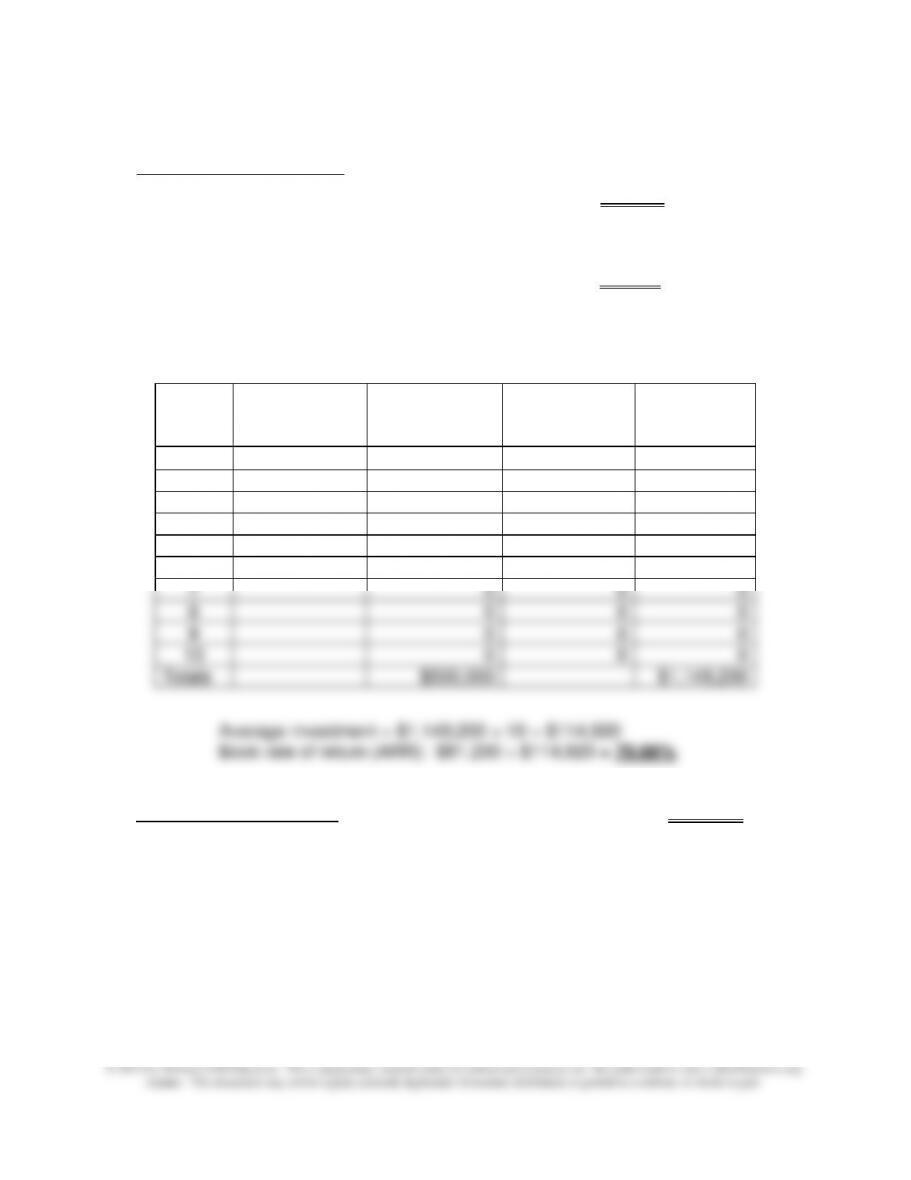
b. On average investment:
Computation of Simple Average Annual Investment:
Average investment: $1,149,200/10 = $114,920
3. Net Present Value (NPV): the NPV of the proposed investment is $229,821 (based
on PV factors from Appendix C, Table 1), as follows:
Year
Book Value,
Beginning-of–
Year
Depreciation
Expense for
the Year
Book Value,
End-of-Year
Average BV
During the
Year
1
$500,000
$100,000
$400,000
$450,000
2
400,000
160,000
240,000
320,000
3
240,000
96,000
144,000
192,000
4
144,000
57,600
86,400
115,200
5
86,400
57,600
28,800
57,600
6
28,800
28,800
0
14,400
7
0
0
0
8
0
0
0
9
0
0
0
10
0
0
0
Totals
$500,000
$1,149,200
Chapter 12 – Strategy and the Analysis of Capital Investments
12–56
12–49 (Continued-2)
Net After-
tax
12%
Present
Value
Cash
Discount
of Net
Year
Inflow
Factor
Cash Inflow
1
$ 65,000
0.893
$ 58,045
2
104,000
0.797
82,888
3
112,800
0.712
80,314
4
157,280
0.636
100,030
5
185,280
0.567
105,054
6
218,640
0.507
110,850
7
189,000
0.452
85,428
8
168,000
0.404
67,872
9
84,000
0.361
30,324
10
28,000
0.322
9,016
Total
$729,821
NPV =
$229,821
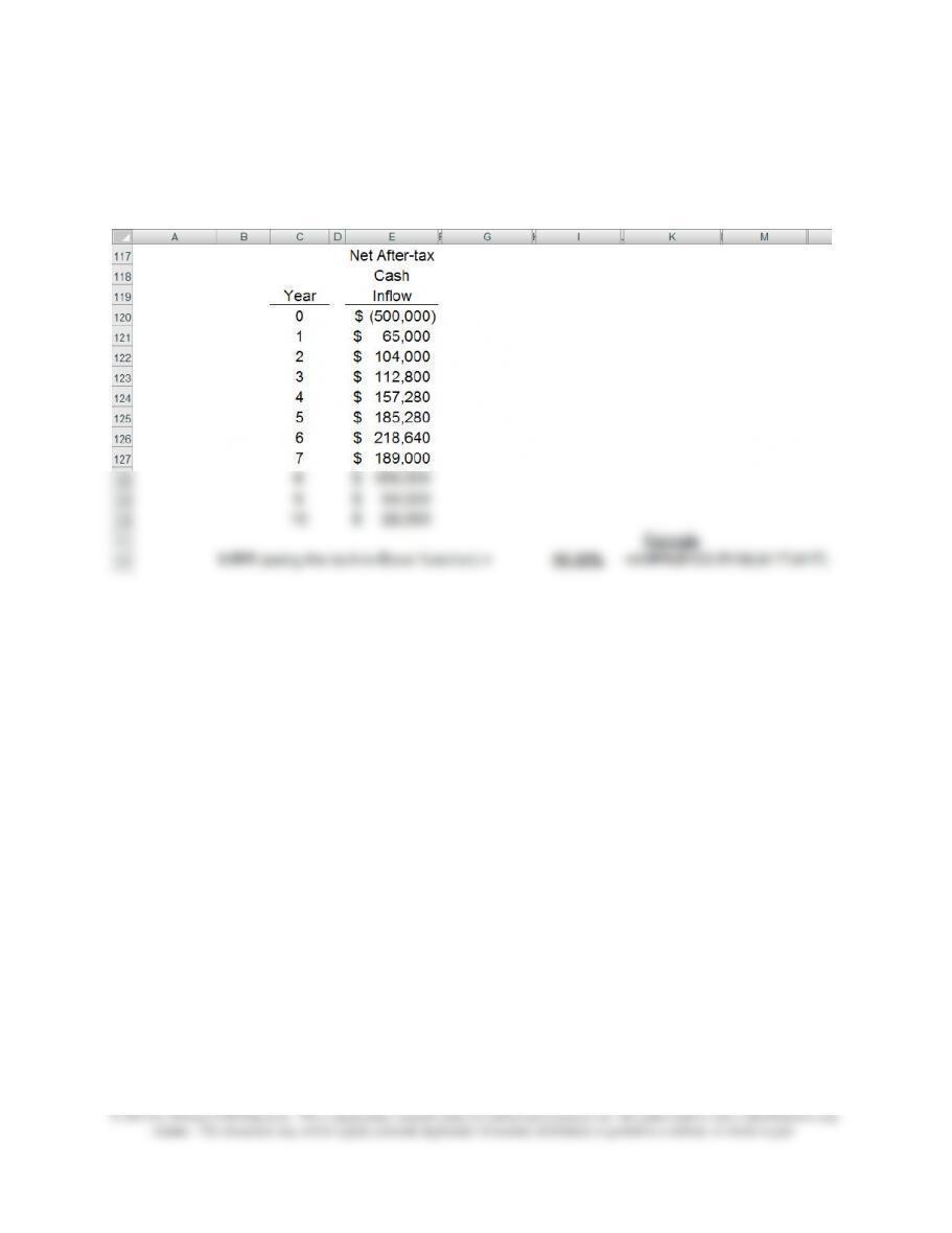
4. Internal Rate of Return (IRR): as indicated in the above schedule, we can use the
built-in function in Excel to estimate the IRR for this proposed investment; IRR =
21.46%.
Chapter 12 – Strategy and the Analysis of Capital Investments
12–57
12–49 (Continued-3)
Thus,
PV
PV
Net After-
20%
of Net
22%
of Net
Year
tax Cash
Inflow
Discount
Factor
Cash
Inflow
Discount
Factor
Cash
Inflow
1
$ 65,000
0.833
$ 54,145
0.820
$ 53,300
2
104,000
0.694
72,176
0.672
$ 69,888
3
112,800
0.579
65,311
0.551
$ 62,153
4
157,280
0.482
75,809
0.451
$ 70,933
5
185,280
0.402
74,483
0.370
$ 68,554
6
218,640
0.335
73,244
0.303
$ 66,248
7
189,000
0.279
52,731
0.249
$ 47,061
8
168,000
0.233
39,144
0.204
$ 34,272
9
84,000
0.194
16,296
0.167
$ 14,028
10
28,000
0.162
4,536
0.137
$ 3,836
$527,875
$490,273
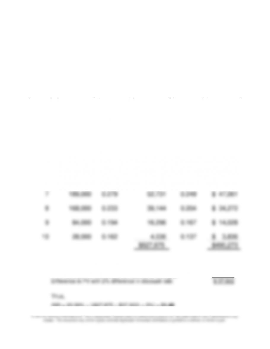
PV of net cash inflows at 20% (a rate that is too low): $527,875
PV of net cash inflows at 22% (a rate that is too high): $490,273
IRR = 20.00% + [($27,875 ÷ $37,602) × 2%] = 21.48
Chapter 12 – Strategy and the Analysis of Capital Investments
12–58
12–49 (Continued-4)
5. Modified internal rate of return (MIRR):
Chapter 12 – Strategy and the Analysis of Capital Investments
12–59
12–50 Real Options (50-60 Minutes)
1. “Real Options” are options embedded in capital investment projects. These options
provide an opportunity for management to dynamically adjust to new information and as
such are analogous to financial options. There are two primary differences between
financial options and real options: (1) the latter involve investments in real assets
(tangible and/or intangible property) while the former relate to financial assets; and (2)
the former are traded on an organized exchange, while the latter are not.
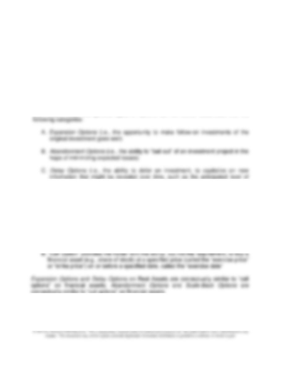
There are, in general, two types of real options: those that provide managerial
flexibility, and those that provide growth options. As noted in the excerpt regarding the
CMA exam, these two general types of options can be further subdivided into the
market demand; these options are also referred to as “wait and see” options)
D. Scale-Back Options (i.e., the ability, through production methods or varying
output, to reduce, but not eliminate, investment in a project)
2. The following two terms are associated with financial options:
A. “Put Option” provides the holder with the ability, but not the requirement, to sell a
given security (e.g., share of stock) at a specified price (called the “exercise price”
or “strike price”) on or before a given date, called the “exercise date”
conceptually similar to “put options” on financial assets.
Chapter 12 – Strategy and the Analysis of Capital Investments
12–60
12–50 (Continued-1)
3. Part a:
Required Investment Outlay, t = 0, $100
Outcome (Demand)
p
Year 1
Year 2
Year 3
NPV of
Outcome
Weighted
NPV
High
0.25
$70
$70
$70
$59.83
$14.96
Medium
0.50
$50
$50
$50
$14.16
$7.08
Low
0.25
$5
$5
$5
($88.58)
($22.15)
1.00
$43.75
$43.75
$43.75
($0.11)
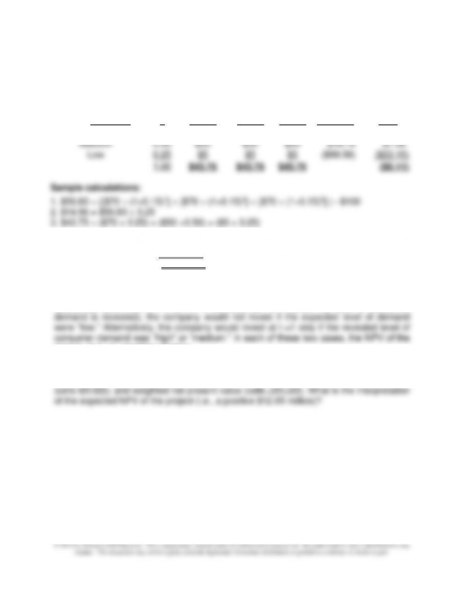
Sample calculations:
1. $59.83 = ([$70 ÷ (1+0.15)1] + [$70 ÷ (1+0.15)2] + [$70 ÷ (1+0.15)3] ) – $100
2. $14.96 = $59.83 × 0.25
3. $43.75 = ($70 × 0.25) + ($50 ×0.50) + ($5 × 0.25)
Part b:
Expected NPV of Project =($108,901) (i.e., ($0.11)*1,000,000, rounded);
Expected NPV of Project =($108,901) (based on PV of stream of $43.75 minus $100)
4. As seen from Part 3 above, the NPV of the project if demand is “low” for each of the
three years would be negative. In Exhibit 12.11, Panel B, this negative amount would be
discounted back from t = 1 to t = 0. As such, at t = 1 (when the level of consumer
project, at t = 1, would be positive.
5. In Panel B of Exhibit 12.11, show for each of the three scenarios the calculation for
present value (at t = 0) of cash inflows (cells H20:H22), present value of cash outflows