Chapter 12 – Strategy and the Analysis of Capital Investments
12–31
12–39 (Continued)
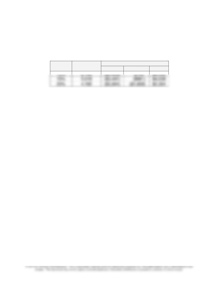
5. NPV Calculations under different assumptions regarding the discount rate
(required rate of return) and annual after-tax net cash inflows. Assume a ten-year
life and an initial investment outlay of $6,000.
15%
5.019
($3,491)
($981)
$4,038
Note to instructor: While this is not required in the present exercise, the above
two-variable “data table” could be generated by using the “Data Table” option under
“What–If Analysis” in Excel 2010. See Problem 12–62 and footnote #17 in Chapter
12.
Discount
PV Annuity
Annual Net After-Tax Cash Flow
Rate
Factor
$500
$1,000
$2,000
10%
6.145
($2,928)
$145
$6,290
20%
4.192
($3,904)
($1,808)
$2,384
Chapter 12 – Strategy and the Analysis of Capital Investments
12–32
12–40 NPV, Sensitivity Analysis (30 minutes)
1. NPV of proposed investment,15-year project life:
PV of after-tax cash inflows = $600,000 × 6.142 = $3,685,200
Initial investment outlay = 3,500,000
NPV of proposed investment, 12-year project life:
PV of after-tax cash inflows = $600,000 × 5.660 = $3,396,000
Initial investment outlay = 3,500,000
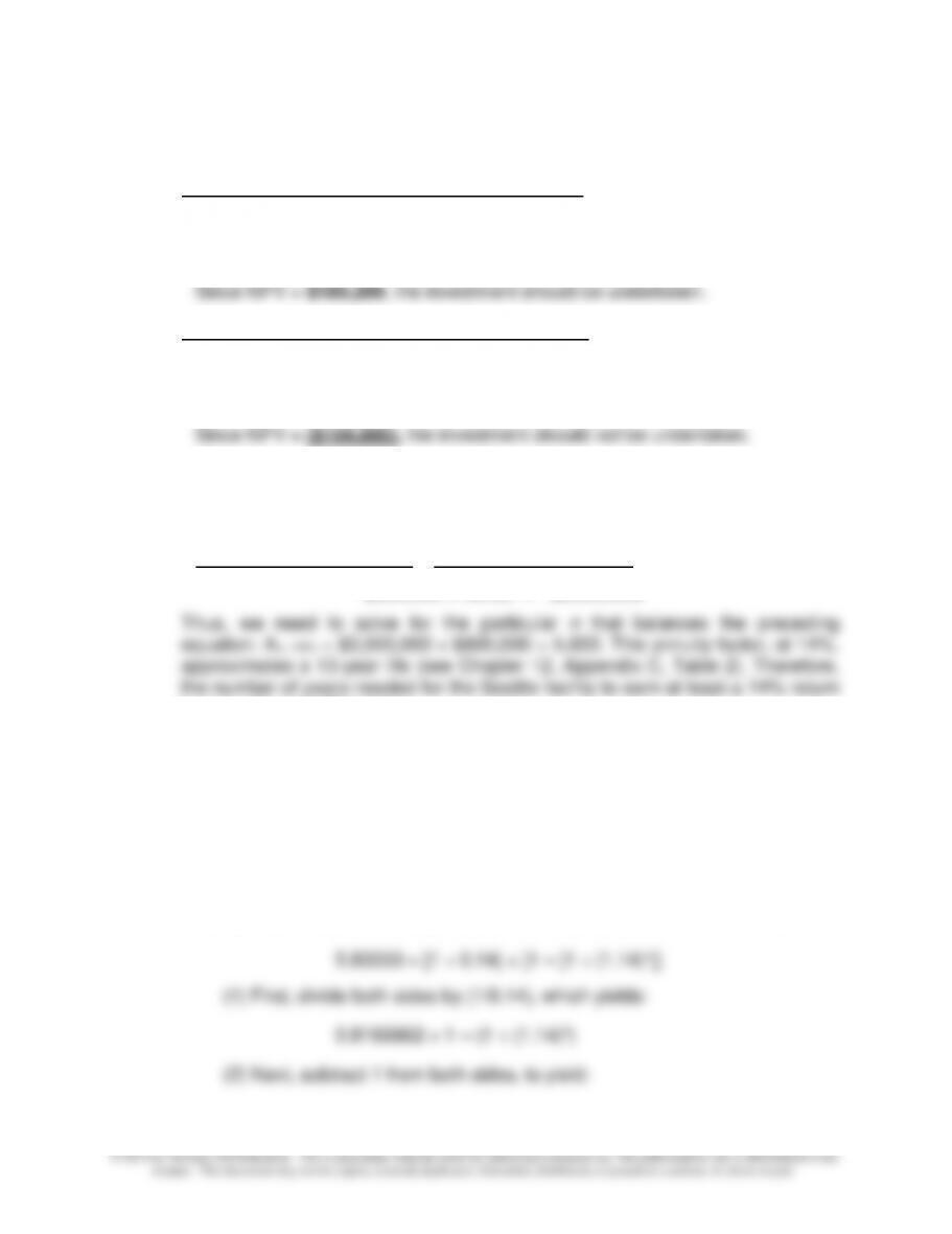
Since NPV = ($104,000), the investment should not be undertaken.
2. We are given annual after-tax cash inflows of $600,000 and an initial
investment outlay of $3,500,000. To generate an IRR of exactly 14.00%, the
following must hold:
PV of Future Cash Inflows = Initial Investment Outlay
$600,000 × An,14% = $3,500,000
is approximately 13 years.
Though not discussed in the text, we can solve exactly for the number of years,
n, once we know the formula to calculate the PV of an ordinary annuity (i.e., the
formula for the factors included in Chapter 12, Appendix C, Table 2). This
formula is:
Annuity Factor = [(1 ÷ r) × [1 – [1 ÷ rn]], where n = the number of periods and
r = the discount rate (defined in terms of n, e.g., in years)
In the present case, the annuity factor = 5.83333 and r = 0.14. Thus, we have
Chapter 12 – Strategy and the Analysis of Capital Investments
12–33
© 2013 by McGraw-Hill Education. This is proprietary material solely for authorized instructor use. Not authorized for sale or distribution in any
manner. This document may not be copied, scanned, duplicated, forwarded, distributed, or posted on a website, in whole or part.
-0.1833338 = – 1 ÷ (1.14)n
12–40 (Continued)
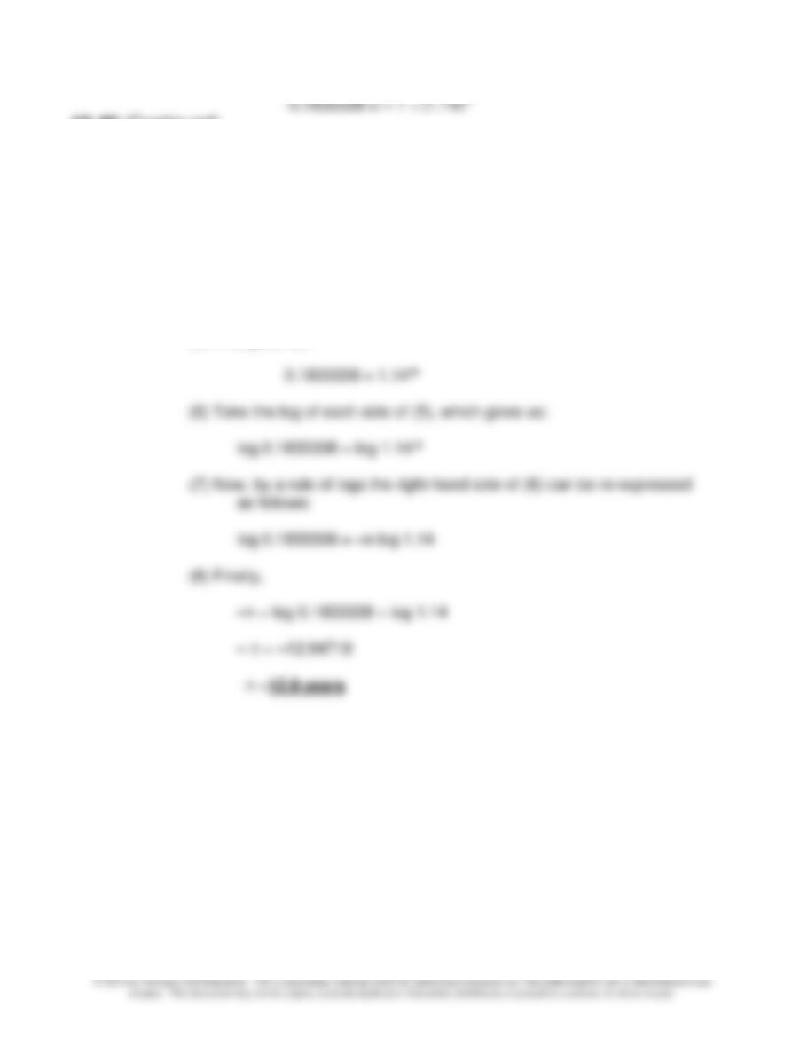
(3) Multiply both sides by –1:
0.1833338 = 1 ÷ (1.14)n
(4) By rule of exponents (i.e., 1 ÷ xn = x-n), the right-hand side of the above
can be expressed as:
1 ÷ (1.14)n= 1.14–n
(5) This gives us:
Chapter 12 – Strategy and the Analysis of Capital Investments
12–34
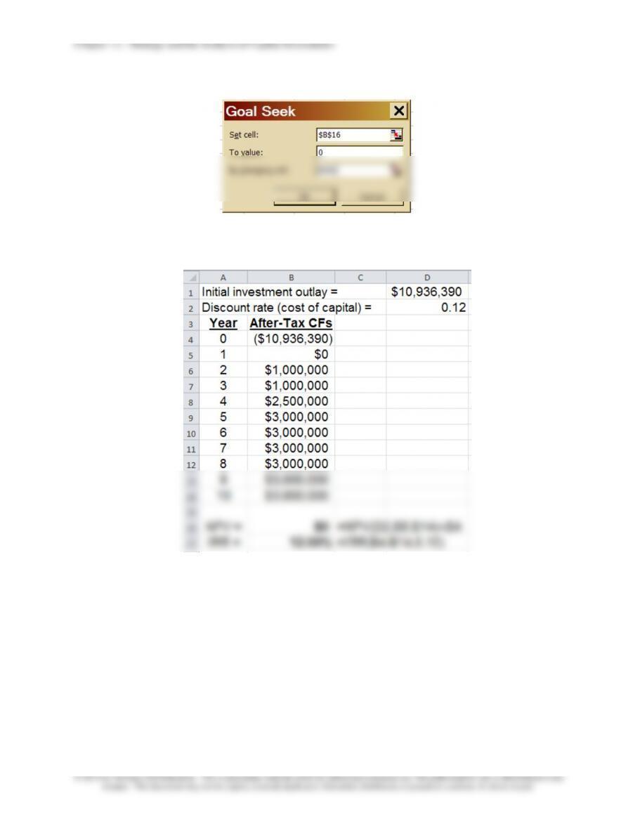
12–41 Uneven Cash Flows, NPV, Sensitivity Analysis (30-40 minutes)
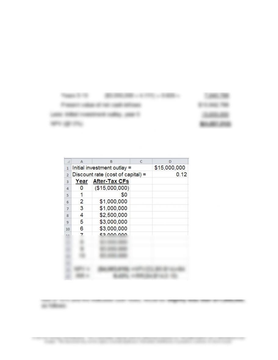
1. Present value of net cash inflows:
Year 1 -0-
Year 2 $1,000,000 × 0.797 = $ 797,000
Year 3 $1,000,000 × 0.712 = 712,000
Year 4 $2,500,000 × 0.636 = 1,590,000
Alternatively, the built-in functions in Excel can be used to estimate the NPV and
the IRR of this project, as follows (Note: the slight difference in answers is due to
rounding—that is, the PV factors in the Tables have been rounded):
2. The maximum purchase price the seller would be willing to offer, given a discount
12–35
12–41 (Continued)
After executing Goal Seek, the following result is obtained for cell D1:
Chapter 12 – Strategy and the Analysis of Capital Investments
12–36
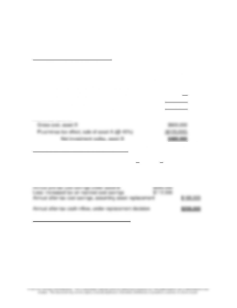
12–42 Asset-Replacement Decision; NPV Analysis (45 Minutes)
1. Relevant (i.e., differential) cash flows (after tax) at:
Project Initiation (i.e., time period 0)
If asset B is purchased, the net investment outlay would be $480,000 (i.e., $600,000
− $120,000).
NBV of existing asset, A
$300,000
Less: Current disposal value of asset A
$0
Gain (Loss) on disposal
($300,000)
Tax effect of sale of existing asset (@ 40%)
($120,000)
Net outlay, asset B:
Gross cost, asset B
$600,000
Plus/minus tax effect, sale of asset A (@ 40%)
($120,000)
Net investment outlay, asset B
$480,000
Project Operation (i.e., years 1-3, inclusive)
A B
Annual depreciation deduction $100,000 $200,000
Annual tax benefit/savings (@40%) $40,000 $80,000
Differential annual tax savings, assuming asset replacement $40,000
Project Termination/Disposal (end of year 3)
N/R—the estimated disposal value of each asset at the end of year 3 is the same, $0,
and therefore not relevant to this asset-replacement decision.
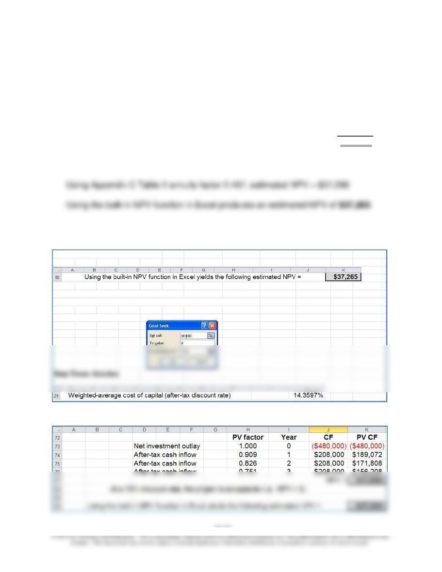
2. Estimated NPV of decision to replace asset A:
Chapter 12 – Strategy and the Analysis of Capital Investments
12–37
12-42 (Continued-1)
PV factor Year CF PV CF
Net investment outlay
1.000
0
($480,000)
($480,000)
After-tax cash inflow
0.909
1
$208,000
$189,072
After-tax cash inflow
0.826
2
$208,000
$171,808
After-tax cash inflow
0.751
3
$208,000
$156,208
NPV =$37,088
At a 10% discount rate, the project is acceptable (i.e., estimated NPV > 0).
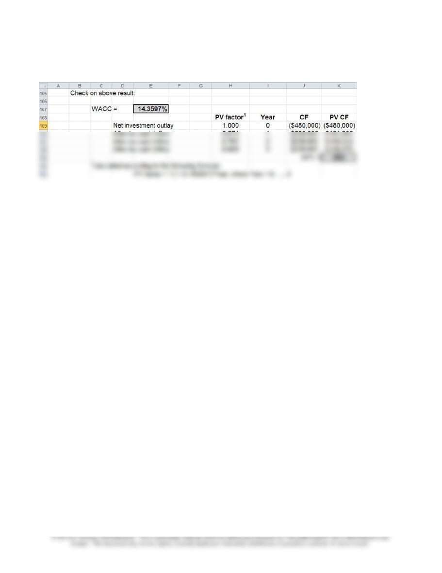
3. The weighted-average cost of capital (WACC) that would make the company
indifferent between keeping or replacing asset A is 14.3597%, as follows:
Step One: Set-up the Problem
Note: the WACC is contained in cell J29
Note: cell K80 contains the formula “=J73+NPV(J29,J74:J76)”
Step Two:Run Goal Seek
Step Three: Solution
The following excerpt is helpful in understanding the above three steps:
Chapter 12 – Strategy and the Analysis of Capital Investments
12–38
12-42 (Continued-2)
12–39
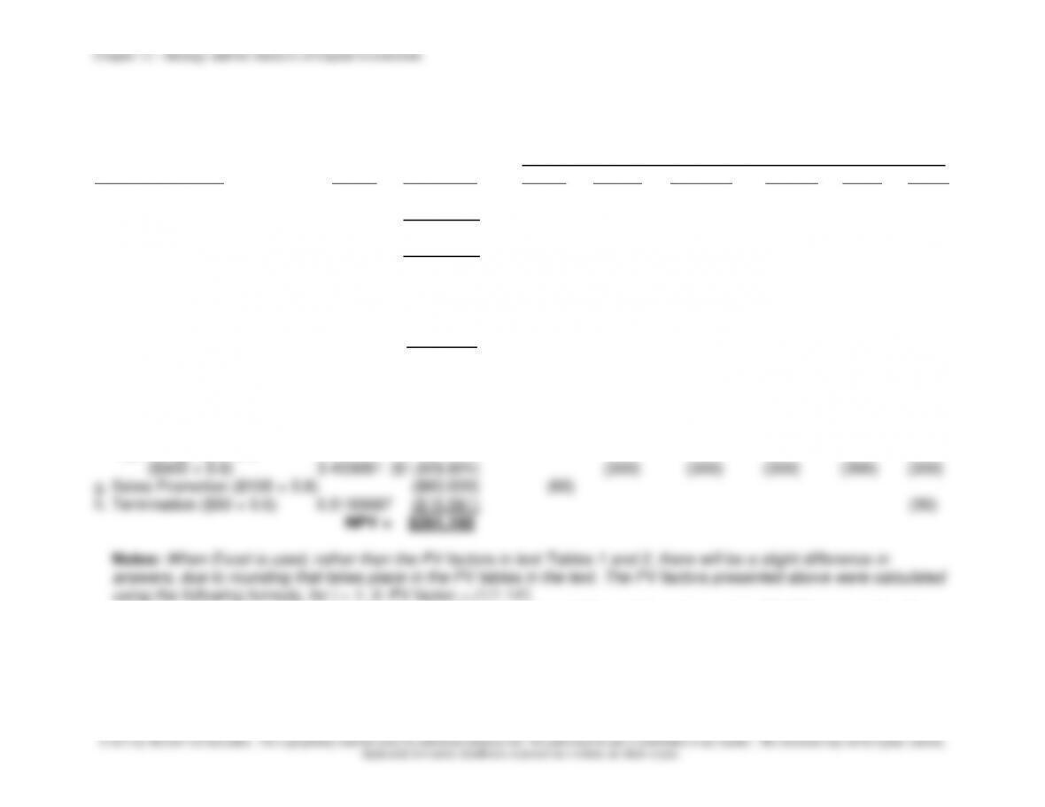
12–43 Cash Flow Analysis; NPV; Spreadsheet Analysis (45 minutes)
1.
PV CASH FLOWS IN YEAR (in ‘000) )
Item & Description Factor PV 0 1 2 3 4 5
a. After-tax rent foregone
($5,000/mo. × 12 × 0.6) N/A ($128,931)1 (36) (36) (36) (36) (36)
b. All are irrelevant
c. Remodeling cost ($100,000) (100)
Depreciation tax savings2 0.877193 $14,035.09 16
0.7694675 $7,386.89 9.6
0.6749715 $3,887.84 5.76
0.5920803 $2,557.79 4.32
0.5193687 $2,243.67 4.32
$30,111 (rounded down)
d. Investment in net working capital ($600,000) (600)
Recovery 0.5193687 $311,621 600
e. Irrelevant
f. Sales ($900 × 0.6) 3.433081 $1,853,864 540 540 540 540 540
Operating expenses
1Use the PV function in Excel to determine the PV of a stream of 60 monthly cash receipts ($3,000 per month, after–
tax). The appropriate formula is: =PV(0.14/12,60,3000).
2Depreciation deductions found using the VDB function in Excel, as follows:
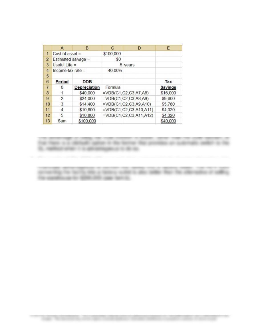
Chapter 12 – Strategy and the Analysis of Capital Investments
12–40
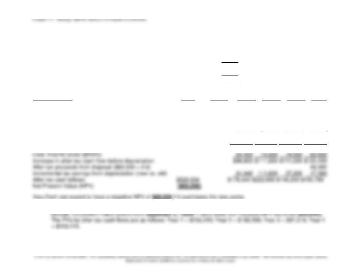
12–43 (Continued)
2. The positive NPV, $261,160, suggests that, compared to the leasing alternative, it is
12–41
© 2013 by McGraw-Hill Education. This is proprietary material solely for authorized instructor use. Not authorized for sale or distribution in any
manner. This document may not be copied, scanned, duplicated, forwarded, distributed, or posted on a website, in whole or part.
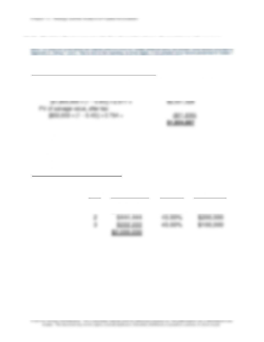
12–44 Machine Replacement with Tax Considerations; Spreadsheet (45 minutes)
and 2 in the text. The solution below is based on the use of PV and NPV functions in Excel.)
Present values of Costs with the Original Equipment:
PV of tax savings from depreciation deductions:
($2,500,000 ÷ 4) × 0.45 × 2.577 = ($724,809) (rounded up)
PV of after-tax cash operating costs:
[$1,800,000 × (1 − 0.45)] × 2.577 = $2,551,326
PV of salvage value, after tax:
[$50,000 × (1 − 0.45)] × 0.794 = ($21,830)
$1,804,687
(NOTE: The present value factors listed above are taken from text Tables 1 and
2 and, as such, have been rounded to three decimal places. However, the actual
calculations above are done using the NPV and PV built-in functions in Excel,
and as such are not rounded.)
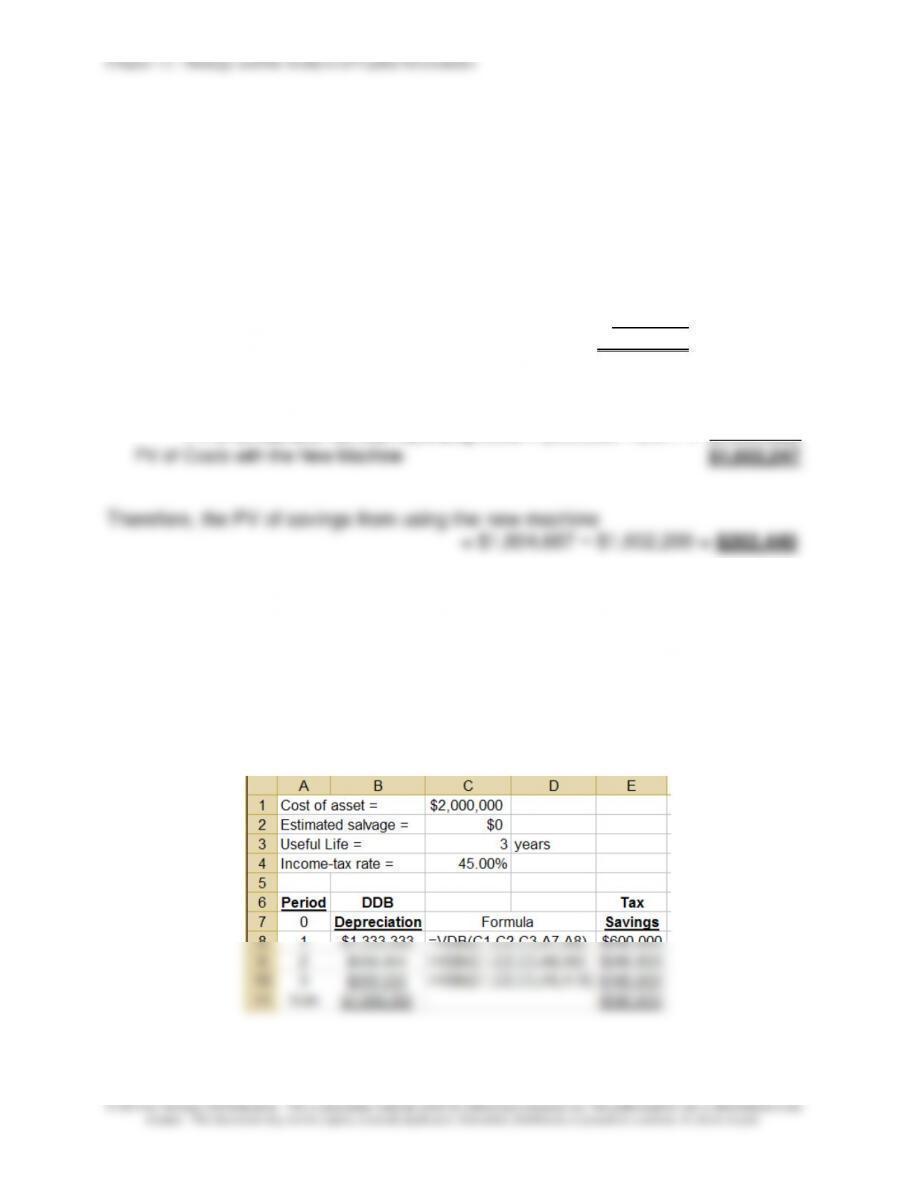
PV of Costs with the New Machine
Present value of tax savings from depreciation deduction:
Year Deprec Expse Tax Rate Tax Savings
0
1 $1,333,333 45.00% $600,000
2 $444,444 45.00% $200,000
3 $222,222 45.00% $100,000
$2,000,000
12–42
12-44 (Continued)
Initial outlay cost, new machine = $2,000,000
PV of tax savings from DDB depreciation (see above) = ($806,407)
Cash proceeds from sale of the old machine = ($300,000)
Tax savings related to loss on disposal of old machine:
($1,875,000 − $300,000) × 0.45 = ($708,750)
Book value of old asset at time of sale:
Original cost of asset (1 year ago) = $2,500,000
Less: accumulated depreciation (1 year) = $625,000
Book value, end of one year = $1,875,000
PV of cash operating costs:
Annual after-tax cash operating costs =
= [$1,000,000 x (1 – 0.45)] = $550,000
PV of annual after-tax cash operating costs = $550,000 × 2.577 =
$1,417,403
PV of Costs with the New Machine $1,602,247
Therefore, the PV of savings from using the new machine
= $1,804,687 − $1,602,200 = $202,440
The total cost of the new machine, including the purchase cost and the cash
operating cost in each of the three years is, in PV terms, $202,440 below the
total cost of continuing with the original equipment. Therefore, from a purely
financial standpoint, the purchase of the new machine is a good investment.
Depreciation Calculations for Replacement Machine: Using VDB Function in
Excel
12–43
12–45 Equipment Replacement; MACRS (50 minutes)
1. Per-unit pre-tax cash flow per unit, additional unit sales:
Sales price per unit $3,500
Current variable (cash) manufacturing cost per unit − 2,450
Current cash contribution margin per unit $1,050
Cash-based cost savings per unit with the new machine + 150
Pre-tax cash flow per unit for the additional units $1,200
After-Tax Cash Flow Analysis Present Discount
Item Description Value Factor1 2016 2017 2018 2019
Purchase cost of the new asset ($608,000)
Capitalized installation cost of the new asset ($12,000)
After-tax proceeds from disposing old ($50,000 × (1 − t)) $30,000
Pre-tax cash flow per unit, sale of add’l units (above) $1,200 $1,200 $1,200 $1,200
Additional units (given) 30 50 50 70
Pre-tax cash flow from additional units $ 36,000 $ 60,000 $ 60,000 $ 84,000
Efficiency savings, pretax 125,000 125,000 125,000 125,000
Total increase in pre-tax cash flow $161,000 $185,000 $185,000 $209,000
1Note: The above PV of after-tax cash inflows ($529,994) was determined using the NPV built-in function in Excel. If,
Chapter 12 – Strategy and the Analysis of Capital Investments
12–44
12–45 (Continued)
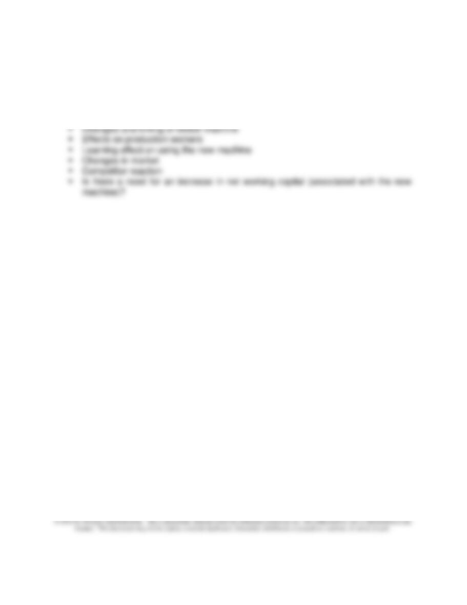
2. Other factors the firm needs to consider include:
▪ Maintenance costs of the machines
▪ Reliability of the machines
Chapter 12 – Strategy and the Analysis of Capital Investments
12–45
12–46 Risk and NPV; Sensitivity Analysis (40-45 minutes)
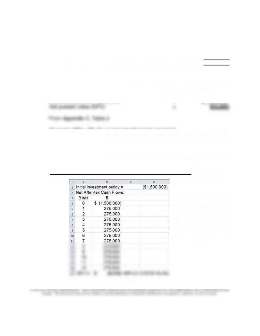
1. PV of future cash inflows: 12 years @ 12% = $275,000 × 6.194* = $1,703,350
Less: Initial investment outlay, year 0 = $1,500,000
Net present value (NPV) = $ 203,350
*From Appendix C, Table 2
Since the NPV > $0, the project should be accepted.
2. PV of future cash inflows @ 15% = $275,000 × 5.421* = $1,490,775
Less: Investment outlay, year 0 = $1,500,000
Since the NPV < $0, the project should not be accepted.
3. The “break–even” initial investment outlay is the amount that would produce a
NPV = $0, given the annual after-tax flows of $275,000 and a discount rate of
15.00%. We can use Excel to solve, in two steps, for this “break–even” amount
(viz., $1,490,670), as follows:
Step 1: Estimate the Project’s NPV (compare with 2 above)