Chapter 12 – Strategy and the Analysis of Capital Investments
12–16
12–30 Future and Present Values Using Excel (30 minutes)
A. To calculate future values, use the following Excel function:
FV(rate,nper,pmt, pv,type)
1. Between January 1, 1701 and December 31, 2012 there are 624 six-month
periods (nper). (624 = ([2012 – 1701] +1) × 2.) Thus, at the end of year 2012,
at an annual interest rate of 6% compounded semiannually, the $24.00 would
have grown to $2,458,325,906, as follows:
FV(0.06/2,624,0,-24,0)
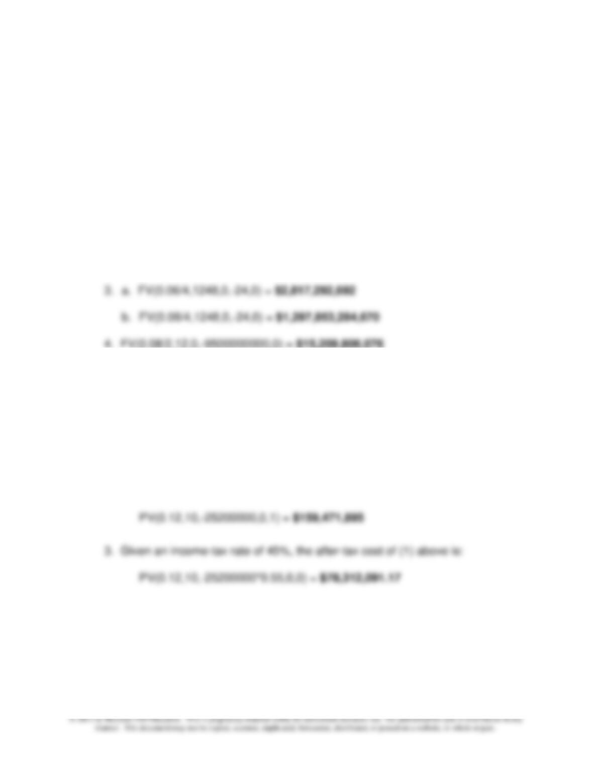
2. FV(0.08/2,624,0,-24,0) = $1,020,974,662,039
B. To calculate present values, use the following Excel function:
PV(rate,nper,pmt,fv,type)
1. For a stream of ten (10) end-of-year payments of $25,200,000 (ordinary
annuity) and a discount rate of 12%, we have:
PV(0.12,10,-25200000,0,0) = $142,385,620
2. If the first payment is received the day the contract is assigned (annuity due),
we have:
Chapter 12 – Strategy and the Analysis of Capital Investments
12–17
12–31 Cash Receipts Frequency and Present-Value Consequences (20 minutes)
1. Periodic cash receipts, to earn a 12% return, if payments are received from the
purchaser for each of the listed situations. NOTE: the PMT function in Excel was
used to generate the periodic cash payment/receipt for each of the following
cases.
PMT(rate,nper,pv,fv,type)
Rate is the interest rate for the loan, nper is the total number of payments, pv is
the present value (i.e., the total amount that a series of future payments is worth
now; also known as the principal), fv is the future value (or a cash balance you
want to attain after the last payment is made; if fv is omitted, it is assumed to be 0
(zero)), and type is the number 0 (zero) or 1 and indicates when payments are
due (if omitted, or 1 is chosen, it is assumed that payments occur at the end of
each period).
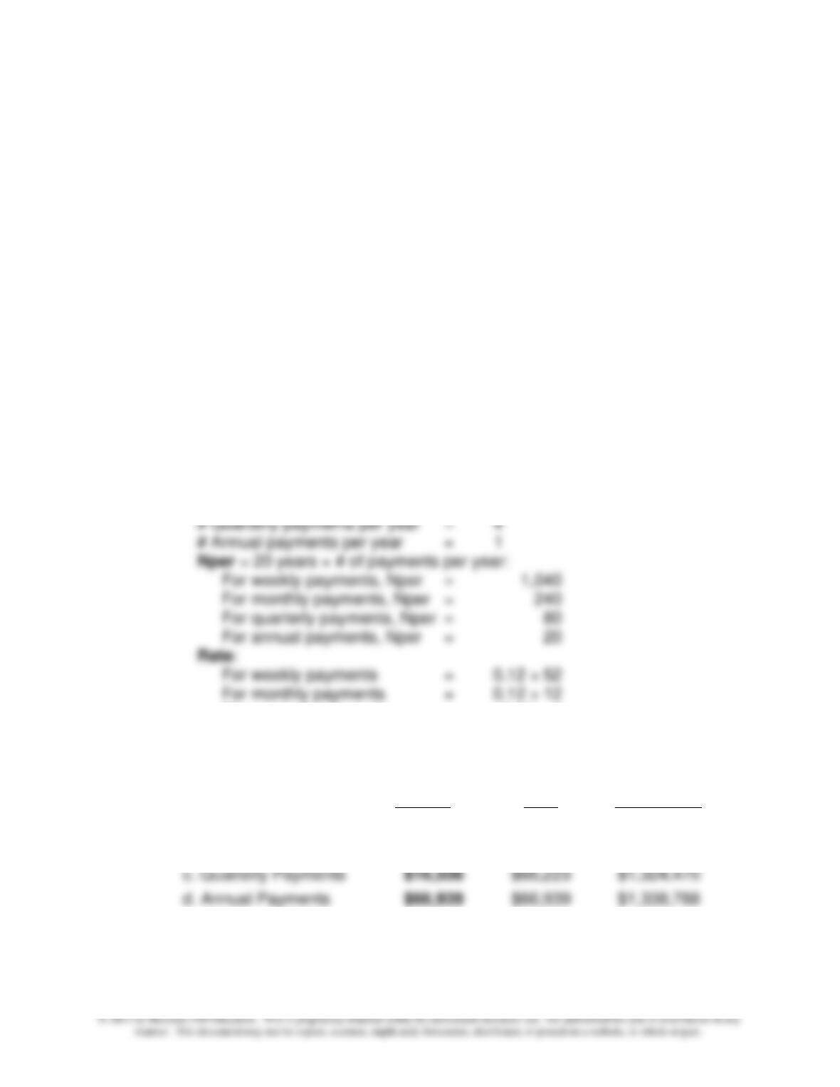
Input Data:
Sales Price (present value, pv) = $500,000
Required Pre-tax Return = 12.00%
Financing Period, years = 20
# Weekly payments per year = 52
# Monthly payments per year = 12
For quarterly payments = 0.12 ÷ 4
For annual payments = 0.12 ÷ 1
Periodic Cash
Receipt
Total per
Year
Total Over 20-
Year Period
a. Weekly Payments
$1,269
$66,004
$1,320,087
b. Monthly Payments
$5,505
$66,065
$1,321,303
c. Quarterly Payments
$16,556
$66,223
$1,324,470
d. Annual Payments
$66,939
$66,939
$1,338,788
12–18
© 2013 by McGraw-Hill Education. This is proprietary material solely for authorized instructor use. Not authorized for sale or distribution in any
manner. This document may not be copied, scanned, duplicated, forwarded, distributed, or posted on a website, in whole or part.
12-31 (Continued)
2. What general conclusion can you draw based on the calculations above in (1)?
Money has a time value. As such, cash received earlier (e.g., on a quarterly basis
rather than an annual basis) has a greater value to the recipient (who, for example,
could invest those receipts). Therefore, when payments are made more frequently, a
lower annual amount will occur. As seen from the data above, total cash
Chapter 12 – Strategy and the Analysis of Capital Investments
12–19
12–32 Value of Accelerated Depreciation (25-30 minutes)
1. The incremental PV of using SYD depreciation rather than SL depreciation, at a
discount rate of 8%, is $1,272, as follows:
PV
Depreciation Method Difference Factor PV of
Year SYD S-L Amount Tax Effect at 8% Tax Effect
1 $40,000 $25,000 $15,000 $6,000 0.926 $5,556
2 30,000 25,000 5,000 2,000 0.857 1,714
3 20,000 25,000 (5,000) (2,000) 0.794 (1,588)
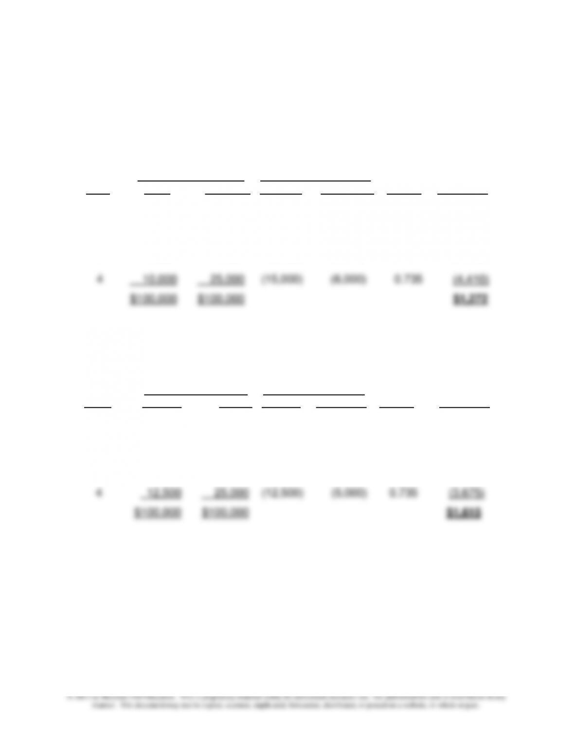
2. The incremental PV of using DDB depreciation rather than SL depreciation, at a
discount rate of 8%, is $1,615, as follows:
PV
Depreciation Method Difference Factor PV of
Year DDB S-L Amount Tax Effect at 8% Tax Effect
1 $50,000 $25,000 $25,000 $10,000 0.926 $9,260
2 25,000 25,000 – 0 – – 0 – 0.857 -0-
3 12,500 25,000 (12,500) (5,000) 0.794 (3,970)
Chapter 12 – Strategy and the Analysis of Capital Investments
12–20
12–32 (Continued)
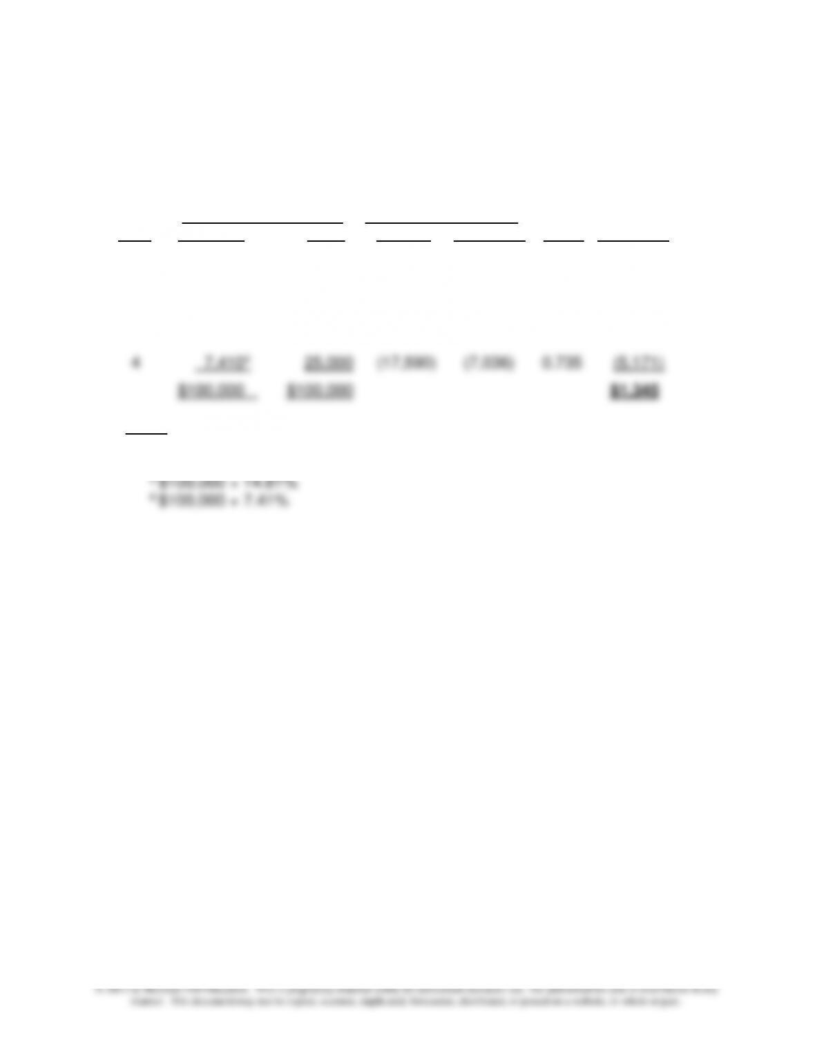
3. The incremental PV of using MACRS depreciation, rather than SL depreciation, at
a discount rate of 8%, is $1,345, as follows:
PV
Depreciation Method Difference Factor PV of
Year MACRS S-L Amount Tax Effect at 8% Tax Effect
1 $33,3301 $25,000 $8,330 $3,332 0.926 $3,085
2 44,4502 25,000 19,450 7,780 0.857 6,667
3 14,8103 25,000 (10,190) (4,076) 0.794 (3,236)
Notes:
1 $100,000 × 33.33%
2 $100,000 × 44.45%
Chapter 12 – Strategy and the Analysis of Capital Investments
12–21
12–33 Weighted-Average Cost of Capital (WACC) (20-25 minutes)
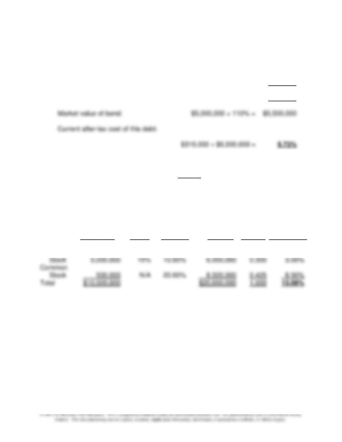
a. Bond interest expense before tax = $5,000,000 × 9% = $450,000
Income tax savings on bond interest expense = $450,000 × 30% = 135,000
After-tax bond interest expense = $315,000
b. After-tax cost of preferred stock = dividend per share/market price per share
= $3 ÷ $30 = 10.00%
c. Using weights based on the current market values of debt and equity, the
estimated WACC for this firm is 13.08%, as follows:
Interest After-tax
or Rate or Current Cost of
Dividend Expected Market Capital
Book Value Rate Return Values Weights Components
Bond $5,000,000 9% 5.73% $5,500,000 0.275 1.58%
Preferred
Chapter 12 – Strategy and the Analysis of Capital Investments
12–22
12–34 Determining Cash Flows; Basic Capital Budgeting (10–15 minutes)
1. The after-tax cash flow from disposal of the old machinery = after-tax gain on
sale = ($1,800 – $0) × (1 – t) = $1,800 × 0.60 = $1,080
2. The PV of after-tax operating cash savings = pre-tax operating cash savings × (1
4. C
Notes:
Chapter 12 – Strategy and the Analysis of Capital Investments
12–23
12–35 After-Tax Net Present Value (NPV) and IRR (non-MACRS rules) (40-45 minutes)
1. a. Net cash inflow each year: $62,000 – $30,000 = $32,000
Present value of net cash inflows (@10%) = $32,000 × 3.170 = $101,440
Therefore, NPV = $101,440 – $60,000 = $41,440
b. Net cash inflow before depreciation $32,000
Depreciation expense ($60,000 ÷ 4 years) 15,000
Increase in net income before tax $17,000
c. Double-declining balance depreciation (non-MACRS):
Beginning Depreciation Accumulated Ending
Year Book Value Expense Depreciation Book Value
0 $60,000
1 $60,000 $30,000 $30,000 30,000
2 30,000 15,000 45,000 15,000
Pre-Tax DDB 30% After-tax 10%
Cash Depreciation Taxable Income Net Cash Discount Present
Year Inflows Expense Income Taxes Inflow Factor Values
0 ($60,000) ($60,000) 1.000 ($60,000)
1 $32,000 $30,000 $ 2,000 $ 600 $31,400 0.909 28,543
2 32,000 15,000 17,000 5,100 26,900 0.826 22,219

Chapter 12 – Strategy and the Analysis of Capital Investments
12–24
12–35 (Continued-1)
2. a. Net cash inflow each year: $62,000 – $30,000 = $32,000
$60,000 = $32,000 × A?, 4
Using the IRR function of Excel, IRR = 39.08%, as follows:
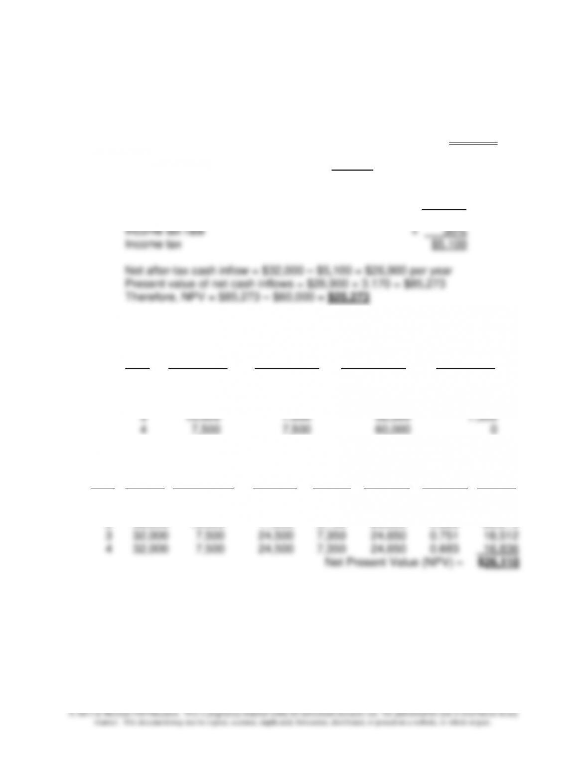
b. Net cash inflow before depreciation $32,000
Depreciation expense ($60,000 ÷ 4 years) 15,000
Increase in net income before tax $17,000
Income tax rate × 30%
Income tax $5,100
Net after-tax cash inflow = $32,000 – $5,100 = $26,900 per year
By inspection of the annuity factors in Appendix C, Table 2, we see that:
We can also use the annuity tables in the text (Appendix C), and interpolation, to
estimate the project’s IRR, as follows:
Discount Rate Discount Factor
25% 25% 2.362 2.362
12–35 (Continued-2)
Chapter 12 – Strategy and the Analysis of Capital Investments
12–25
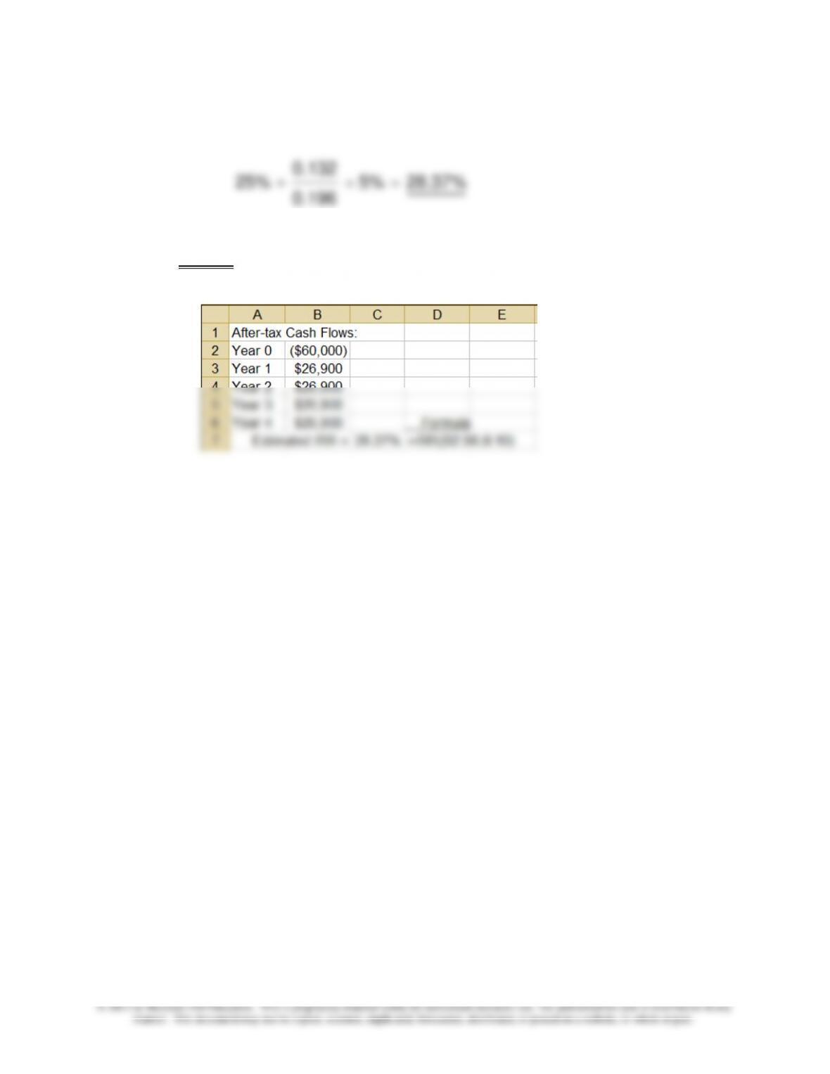
Therefore, estimated Internal Rate of Return (IRR) =
Finally, we could use the built-in IRR function in Excel, which provides an IRR
= 28.27%, as follows:
Chapter 12 – Strategy and the Analysis of Capital Investments
12–26
12-36 Using Arrays in Excel; NPV Analysis (45minutes)
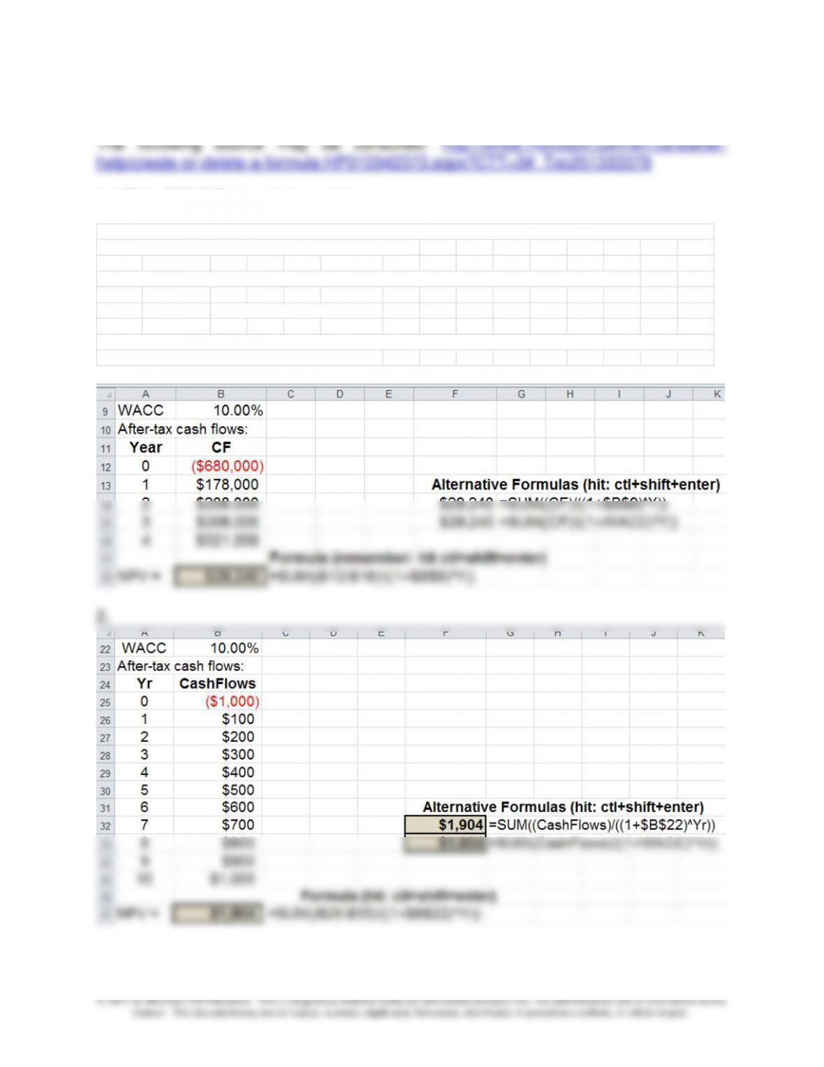
1. NPV = $29,240 (rounded), as follows:
First, define variable names (go to “Formulas,” then “Define Names“). For example, define cell B9 as “WACC,” cells A12
through A16 as “Year,” and cells B12 through B16 as “CF.”
Next, enter into an open cell (e.g., B18) the following formula to calculate the estimated NPV of this project:
=SUM(CF/(1+WACC)^Year)
Finally, rather than hitting “enter,” you now hit the following (to enter the array formula): control+shift+enter. Cell B18 should
now display the correct amount, $29,240 (rounded).
12–37 Basic Capital Budgeting Techniques (45-50minutes)
a. Project A:
b. Project B:
After-tax Cumulative
Year Cash Inflows After-tax Cash Inflows
1 $ 500 $ 500
2 1,200 1,700
3 2,000 3,700
4 2,500
c. Project C:
Depreciation expense per year: $5,000 ÷ 5 = $1,000
Taxable income each year: $2,500 – $1,000 = $1,500
Income tax each year: $1,500 × 25% = $375
Annual after-tax net cash inflow: $2,500 – $375 = $2,125
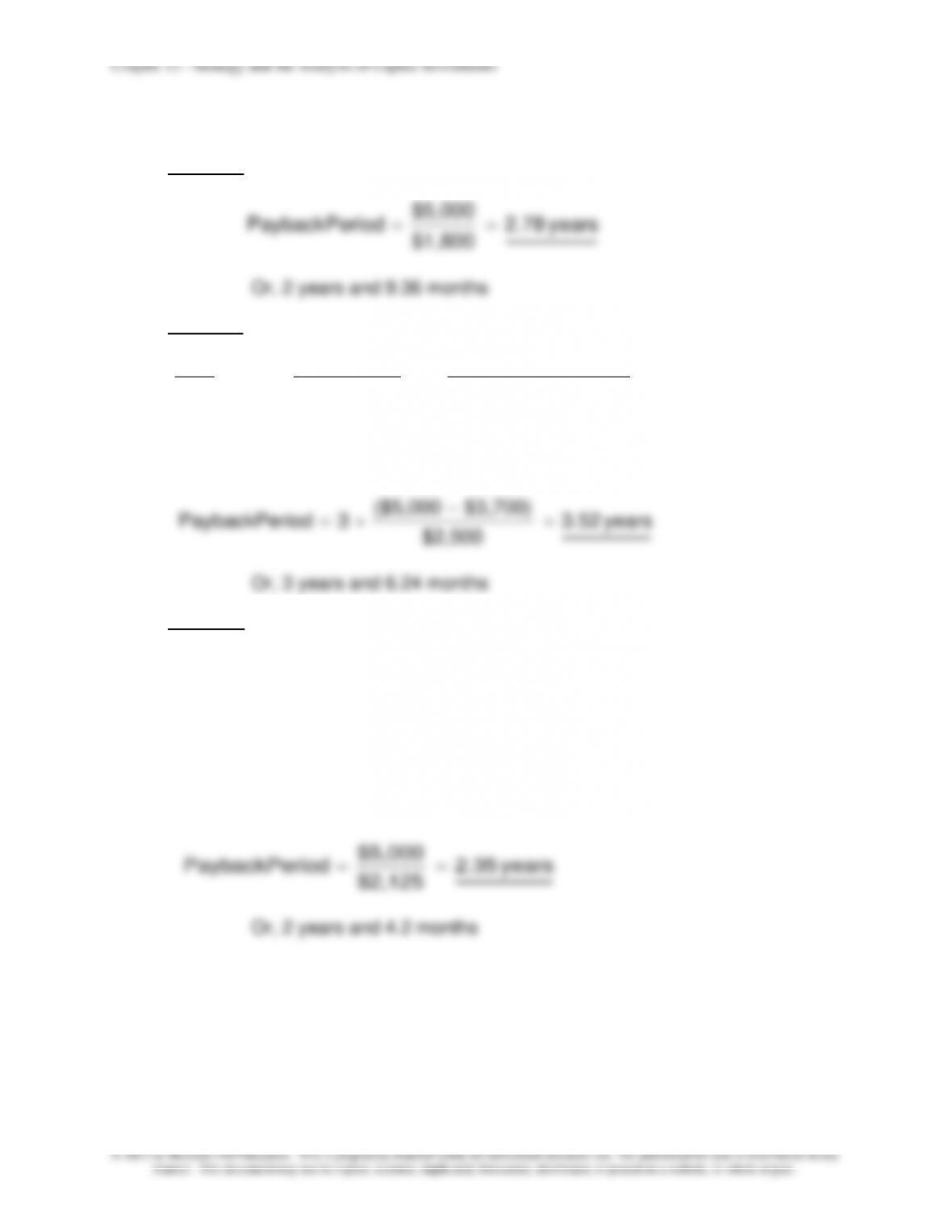
years2.78
$1,800
$5,000
PeriodPayback ==
years3.52
$2,500
$3,700)($5,000
3PeriodPayback =
−
+=
Chapter 12 – Strategy and the Analysis of Capital Investments
12–28
d. Project D:
(1) Depreciation expense per year: ($5,000 – $500) ÷ 5 = $900
Taxable income:
Sales $4,000
Expenses:
Cash expenditures $1,500
Depreciation 900 2,400
Operating income before tax $1,600
Income tax (25%) 400
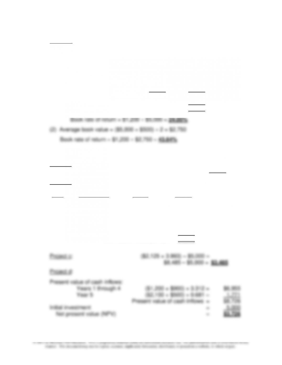
Operating income after tax $1,200
e. Net Present Values (@8%), rounded:
Project a: ($1,800 x 3.993) – $5,000 =
$7,187 – $5,000 = $2,187
Project b:
After-tax 8% Discount Present
Year Cash Flows Factor Values
0 <$5,000>
1 $ 500 0.926 463
2 1,200 0.857 1,028
3 2,000 0.794 1,588
4 2,500 0.735 1,838
5 2,000 0.681 1,362
Net Present Value (NPV) = $1,279
Chapter 12 – Strategy and the Analysis of Capital Investments
12–29
12–38 Straightforward Capital Budgeting with Income Taxes (Non-MACRS-based
Depreciation) and Sensitivity Analysis (20-25 minutes)
1. Depreciation per year, SL basis: ($30,600 – $600) ÷ 6 years = $5,000
Taxable income $8,000 – $5,000 = 3,000
Tax rate × 40%
Income taxes $1,200
2. Payback period: $30,600 ÷ $5,000* = 6.12 years (if cash flows are assumed to
*Given/assumed.
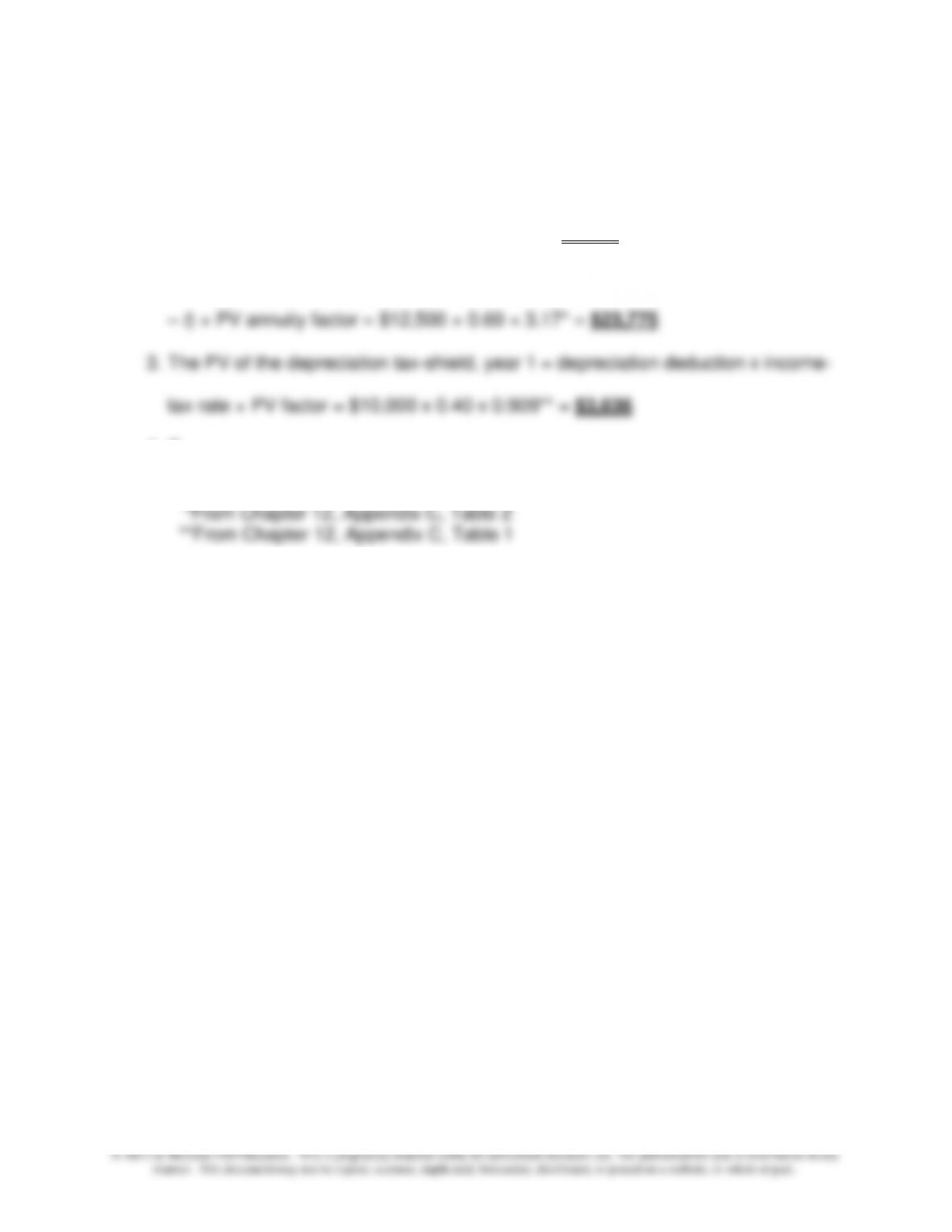
3. PV of annual after-tax cash savings $5,000 × 4.623* = $23,115
PV of salvage value $ 600 × 0.63** = 378
*From Appendix C, Table 2
**From Appendix C, Table 1
4. The minimum net after-tax annual cost savings needed to justify this investment =
$6,537
Let X = minimum after-tax annual cost savings, and let NPV = 0. The Initial
Investment Outlay ($30,600) is reduced by the PV of the salvage value of the asset
@ an 8% discount rate (i.e., $378). Thus, when NPV = $0, we have (by definition):
PV of After-tax Cash Inflows = PV of Cash Outflows
(or, an increase of approximately 31% over the $5,000 amount given assumed
above in 2 and 3)
Chapter 12 – Strategy and the Analysis of Capital Investments
12–30
12-39 Capital Budgeting with Tax, Non-MACRS Depreciation, and Sensitivity
Analysis (30-35 minutes)
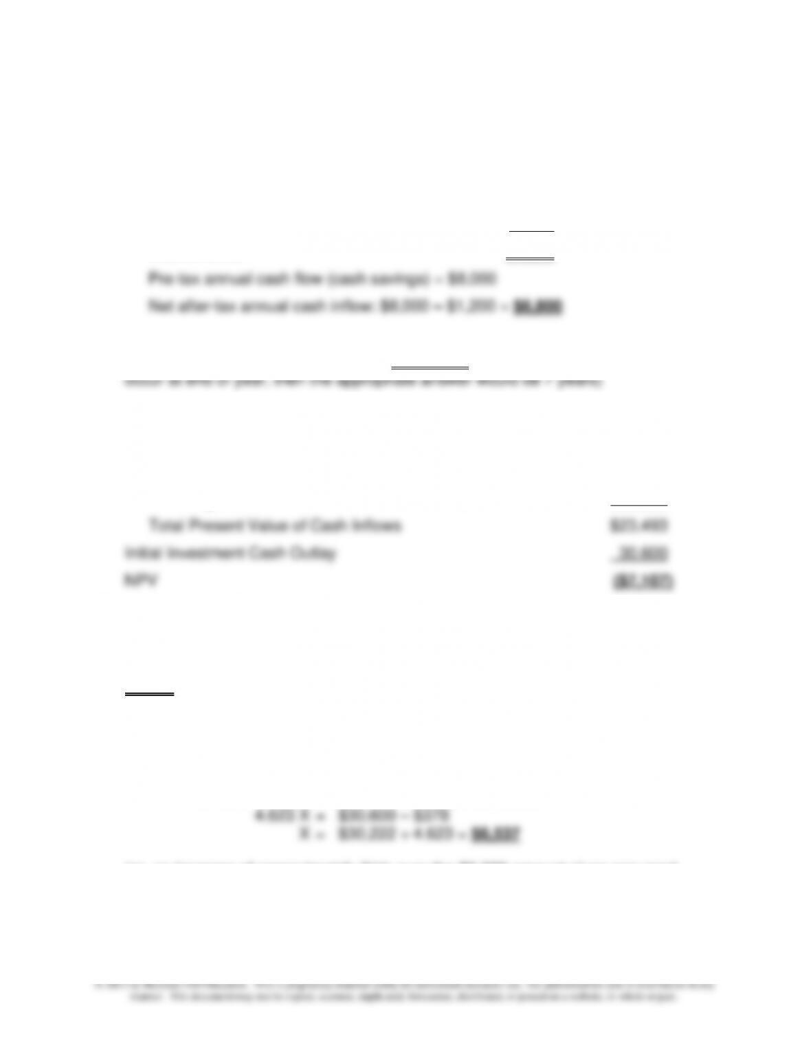
Annual after-tax net cash inflow:
Cash revenue, net of tax $1,200 × (1 – 0.35) = $780
1. Under the assumption that the cash inflows occur evenly throughout the year,
the payback period for the proposed investment is:
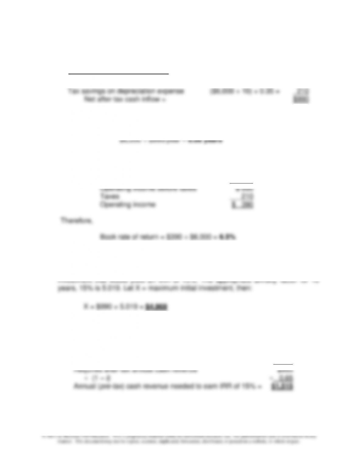
2. Estimated Operating Income per year:
Sales $1,200
Depreciation 600
3. The maximum initial investment is such that the project at
this level of investment would yield a NPV = $0 (i.e., a situation where PV of cash
inflows = PV of cash outflows). Alternatively, we’re looking for the maximum level of
4. Required annual (pre-tax) cash revenue:
Given an initial investment outlay of $6,000, the after-tax
annual cash flow needed per year to generate a return
of 15% = $6,000 ÷ 5.019 = $1,195
Less: Annual Tax savings on depreciation expense = 210