Chapter 11 – Decision Making with a Strategic Emphasis
11–76
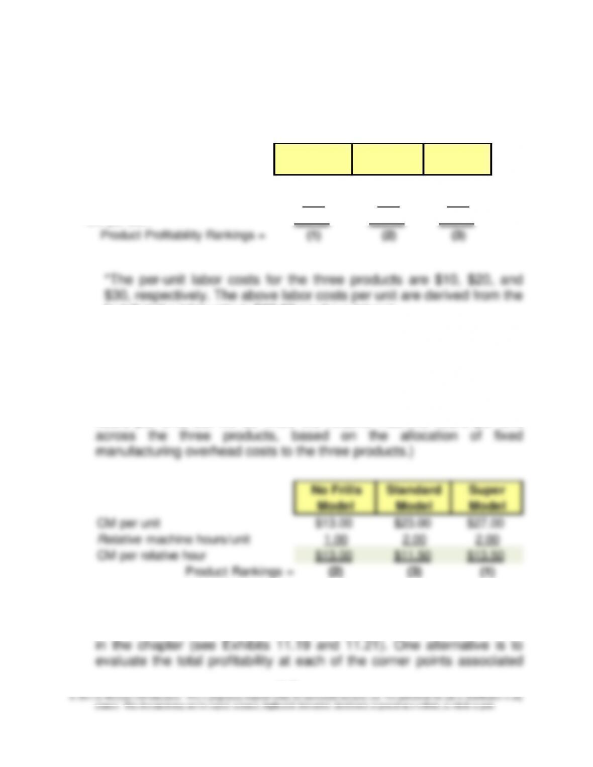
Product Rankings =
(2) (3) (1)
11-44 (Continued-1)
fact that the labor rate is $20.00 per hour (given).
4. If machine hours represent the scarce resource, then the allocation of
machine hours to products should be based on the contribution margin
per machine hour. As seen from the calculations below, the product
profitability rankings differ from those determined in Part 3 above.
(Note that in the present case we do not know the actual machine
hours per unit, but we do know the relative machine hours per unit
5. If there are only two products (and one or more constraints), we could
solve the product-mix problem using the graphical approach presented
No Frills Standard Super
Model Model Model
CM per unit $13.00 $23.00 $27.00
÷ DLHs/unit of output* 0.50 1.00 1.50
CM per DLH $26.00 $23.00 $18.00
Chapter 11 – Decision Making with a Strategic Emphasis
11–77
with the feasible region and to choose the product mix (corner point)
that maximizes short-term profit. Another alternative is to us a set of
iso-profit lines (combination of the two products that results in a given
level of profit). Extend the iso-profit line up to the right until it just
11-44 (Continued-2)
touches a point in the feasible set (region): this point (mix of the two
products) defines the optimum product mix.
6. In the case where there are more than two products (and one or more
constraints), the graphical approach is not practical. In this case, the
7. The primary role of the management accountant in terms of short-term
profit planning is to generate accurate estimates of the contribution
margins for each product (or service). Whether a simple or a complex
decision context, the general solution to the product-mix problem is to
11–78
© 2013 by McGraw-Hill Education. This is proprietary material solely for authorized instructor use. Not authorized for sale or distribution in any
manner. This document may not be copied, scanned, duplicated, forwarded, distributed, or posted on a website, in whole or part.
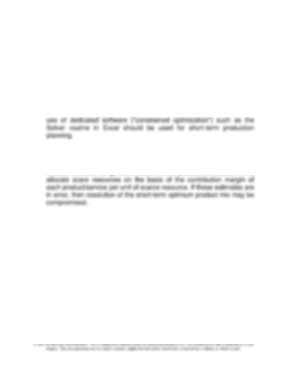
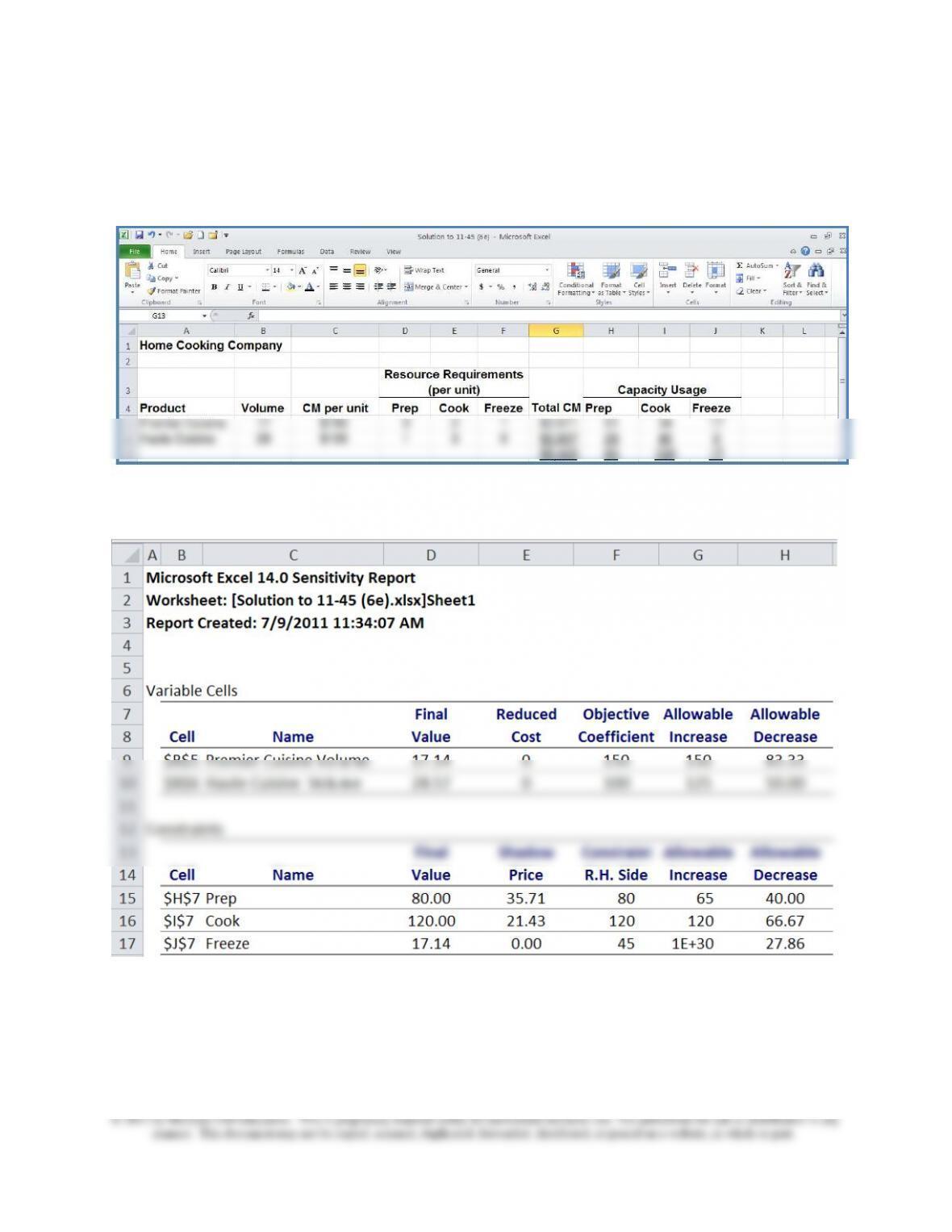
11–45 Profitability Analysis; Linear programming (50-60 min)
1. Solve for all three constraints: the solution is 17 units of Premier
Cuisine and 29 units of Haute Cuisine, as shown in Exhibit 11-45C,
cells B5 and B6. Total contribution margin for this mix is $5,429. The
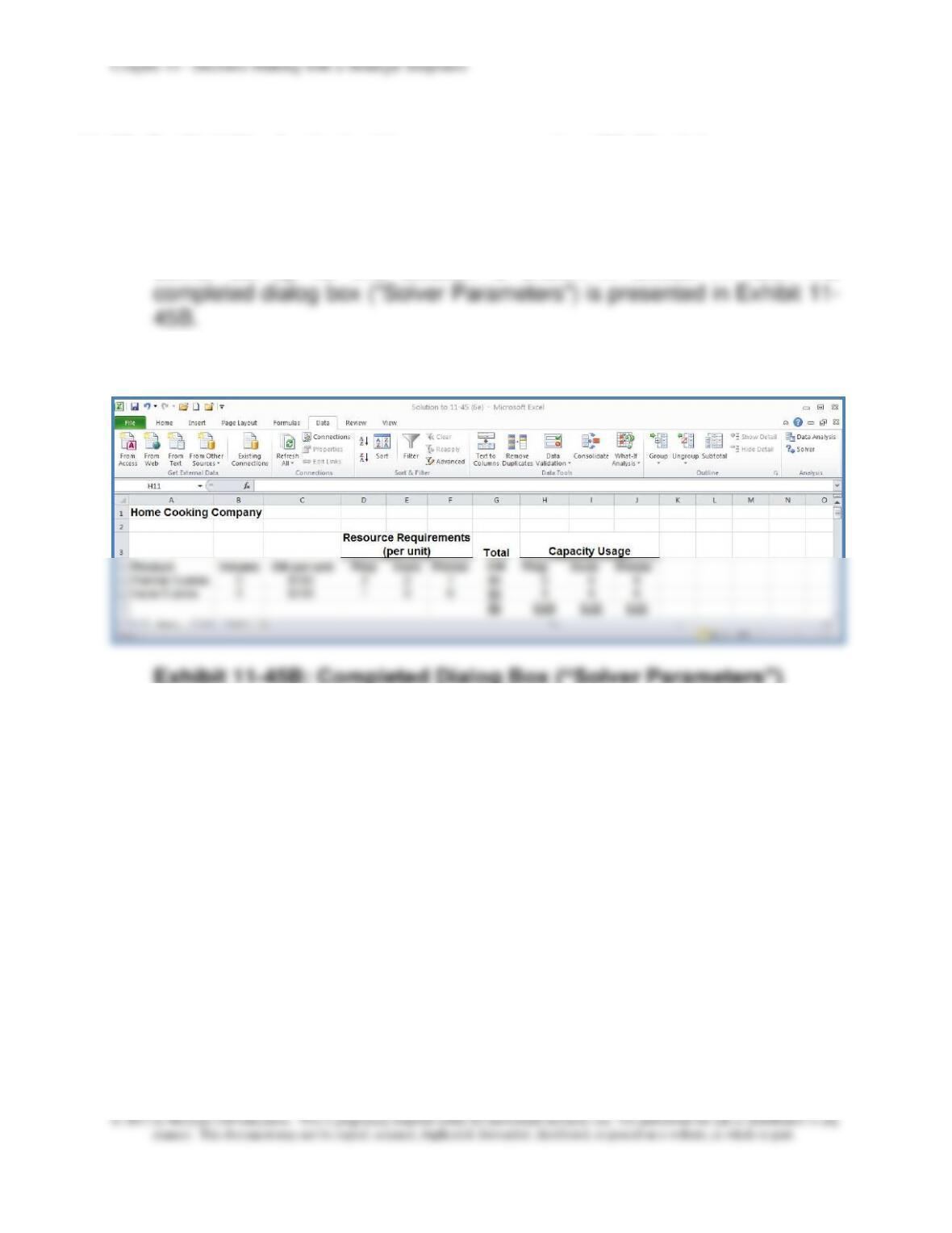
Solver set up for this solution is shown in Exhibit 11–45A. The
Exhibit 11-45A: Solver Set Up
Exhibit 11-45B: Completed Dialog Box (“Solver Parameters”)
Chapter 11 – Decision Making with a Strategic Emphasis
11–79
Chapter 11 – Decision Making with a Strategic Emphasis
11–80
11-45 (Continued-1)
Exhibit 11-45C: Solver Solution (Optimum Product Mix)
2. Sensitivity Report
Notes—Sensitivity Report:
Chapter 11 – Decision Making with a Strategic Emphasis
11–81
1. Reduced costs: these pertain to the two decision variables (Premier
and Haute). If all such variables are in the optimum solution (as in the
present case), then these values will all be zero. Technically, the
11-45 (Continued-2)
“reduced cost” for a variable not in the optimum solution represents
the amount by which the per-unit contribution margin would have to
change in order for the variable to enter the optimal solution.
2. For each decision variable, the “Allowable Increase” and “Allowable
Decrease” provide a range over the objective function coefficients
(here, per-unit contribution margins) over which the optimum solution
willing to pay for one additional unit (here, hour) of each constraint.
You will note that under the optimum solution the entire amount of
Freeze hours is not used up. Thus, by definition the “shadow price”
for this constraint must be zero.
4. Finally, for each constraint there is an “Allowable Increase” and an
“Allowable Decrease.” This information shows the range, around the
value of each constraint, over which the indicated “shadow prices”
hold.
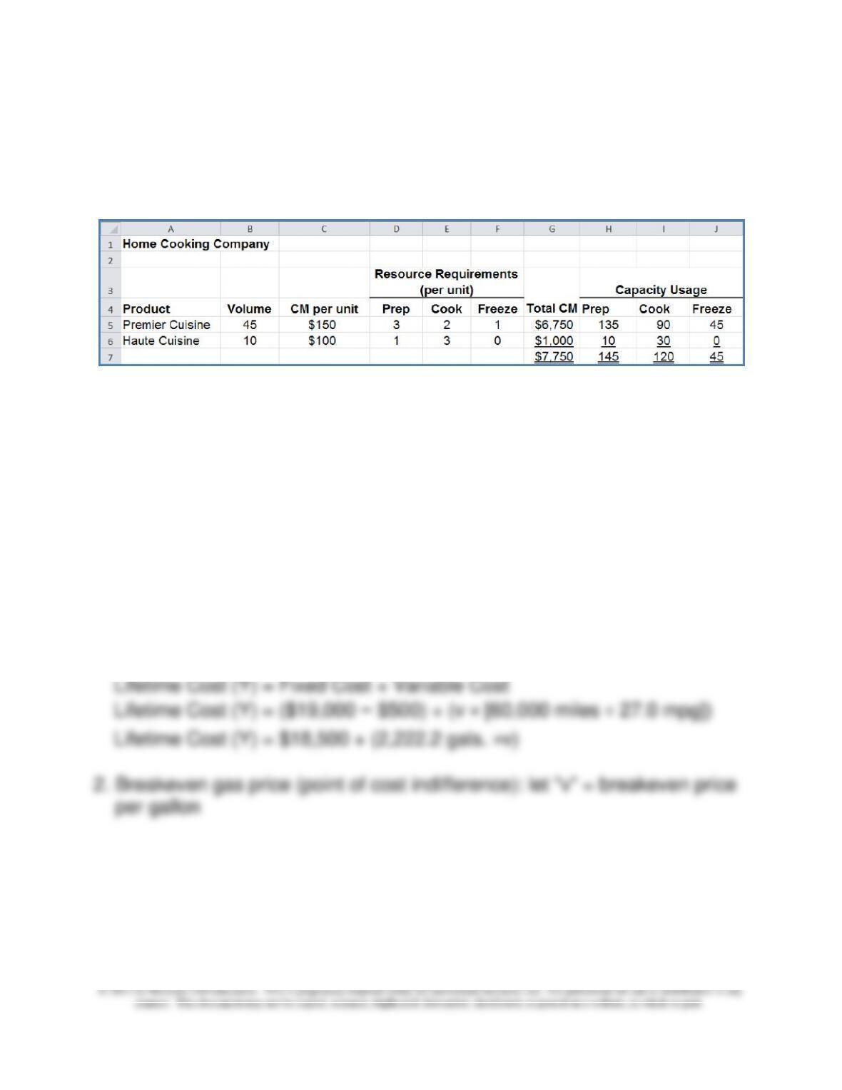
3. Optimal Solution after removing preparation time constraint: the optimal
Chapter 11 – Decision Making with a Strategic Emphasis
11–82
11-45 (Continued-3)
Exhibit 11-45D
11–46 (Also Problem 9-50): CVP Analysis; Sustainability; Uncertainty;
Decision Tables (60-75 min)
1. Lifetime cost functions: let Y = lifetime cost, and v = cost per gallon of
gas
Regular model:
Lifetime Cost (Y) = Fixed Cost + Variable Cost
Lifetime Cost (Y) = $17,000 + (v × [60,000 miles ÷ 23.0 mpg])
Lifetime Cost (Y) = $17,000 + (2,608.7 gals. × v)
Hybrid model:
Lifetime Cost (Y) = Fixed Cost + Variable Cost
Lifetime Cost (Y) = ($19,000 − $500) + (v × [60,000 miles ÷ 27.0 mpg])
Lifetime Cost (Y) = $18,500 + (2,222.2 gals. ×v)
2. Breakeven gas price (point of cost indifference): let “v” = breakeven price
per gallon
Chapter 11 – Decision Making with a Strategic Emphasis
11–83
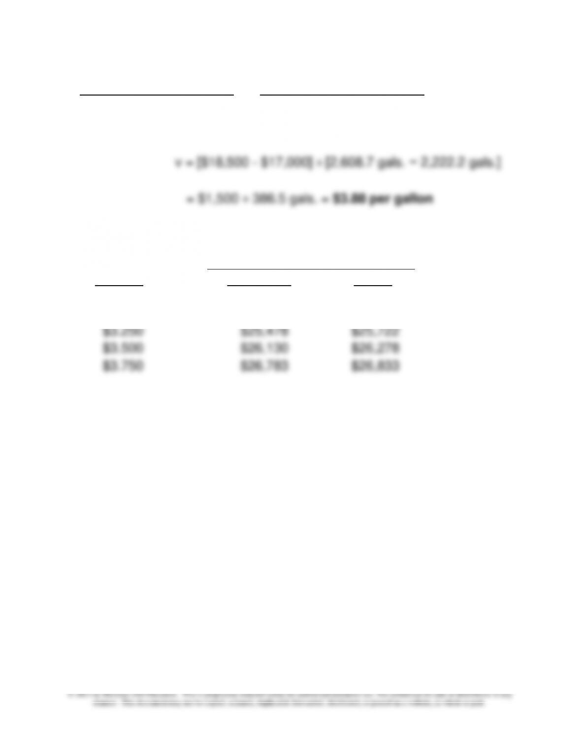
Lifetime Cost—Gas Model = Lifetime Cost—Hybrid Model
$17,000 + (2,608.7 gals. × v) = $18,500 + (2,222.2 gals. × v)
v = [$18,500 – $17,000] ÷ [2,608.7 gals. − 2,222.2 gals.]
= $1,500 ÷ 386.5 gals. = $3.88 per gallon
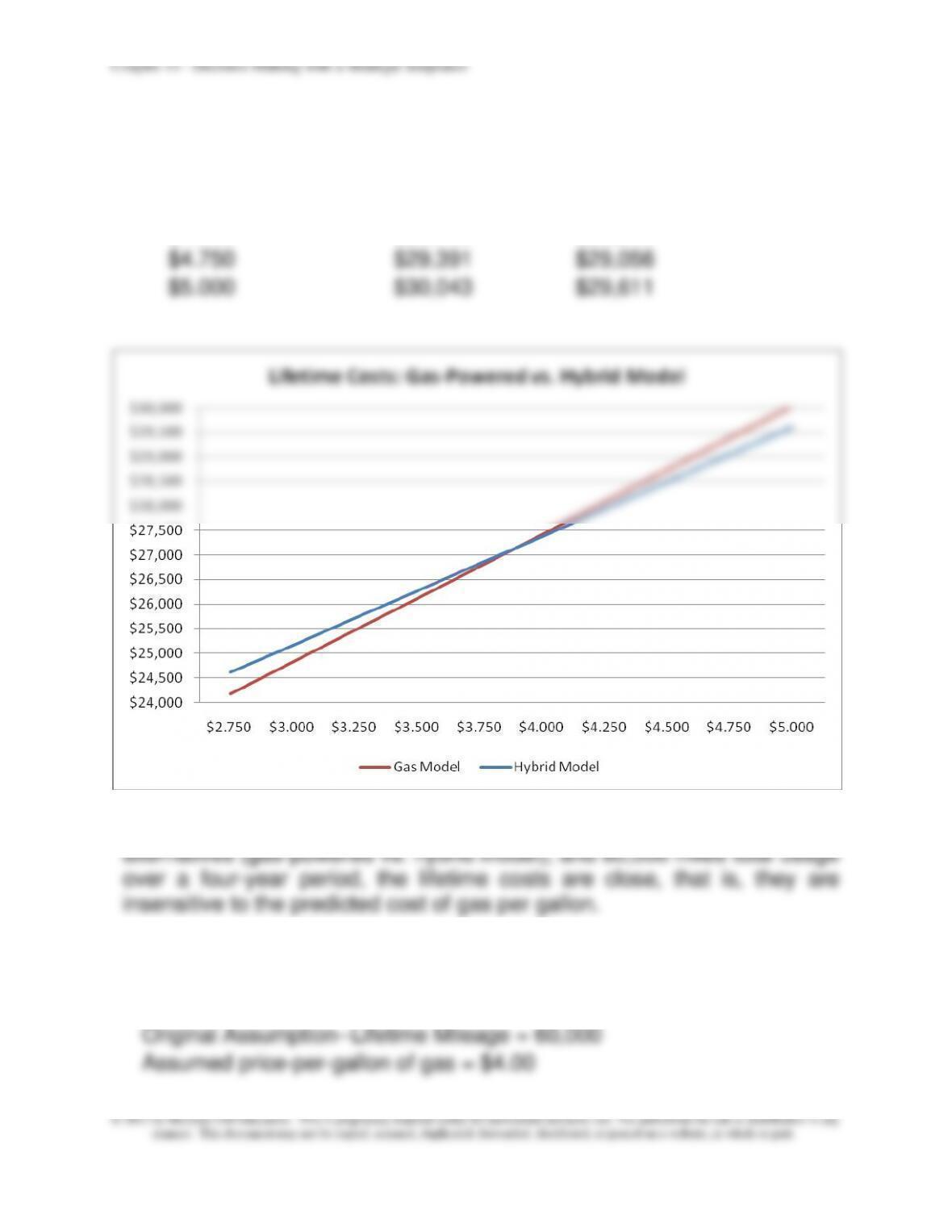
3. Graph of Lifetime Cost Function—Regular and Hybrid Models
X (price
Lifetime Cost
per gal.)
Gas Model
Hybrid
$2.750
$24,174
$24,611
$3.000
$24,826
$25,167
$3.250
$25,478
$25,722
$3.500
$26,130
$26,278
$3.750
$26,783
$26,833
11–84
11–46 (Continued-1)
$4.000
$27,435
$27,389
$4.250
$28,087
$27,944
$4.500
$28,739
$28,500
$4.750
$29,391
$29,056
$5.000
$30,043
$29,611
Based on the above analysis and graph, we see that for these two
4. Pseudo degree of operating leverage (DOL) measure
Alternative Lifetime Mileage Assumption = 62,000
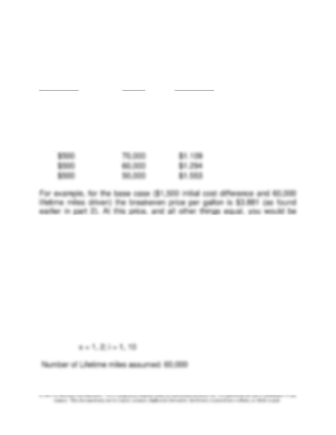
Original Assumption—Lifetime Mileage = 60,000
Assumed price-per-gallon of gas = $4.00
Chapter 11 – Decision Making with a Strategic Emphasis
11–46 (Continued-2)
Lifetime Cost
Lifetime Cost
%
Option
@ 62,000
miles
@ 60,000
miles
Change
Cost
% Change
Mileage
Pseudo
DOL
Gas Powered
Car
$27,783
$27,435
1.2678%
3.333%
0.380
Hybrid Model
$27,685
$27,389
1.0818%
3.333%
0.325
The above pseudo DOL measure for the gas-powered car indicate that
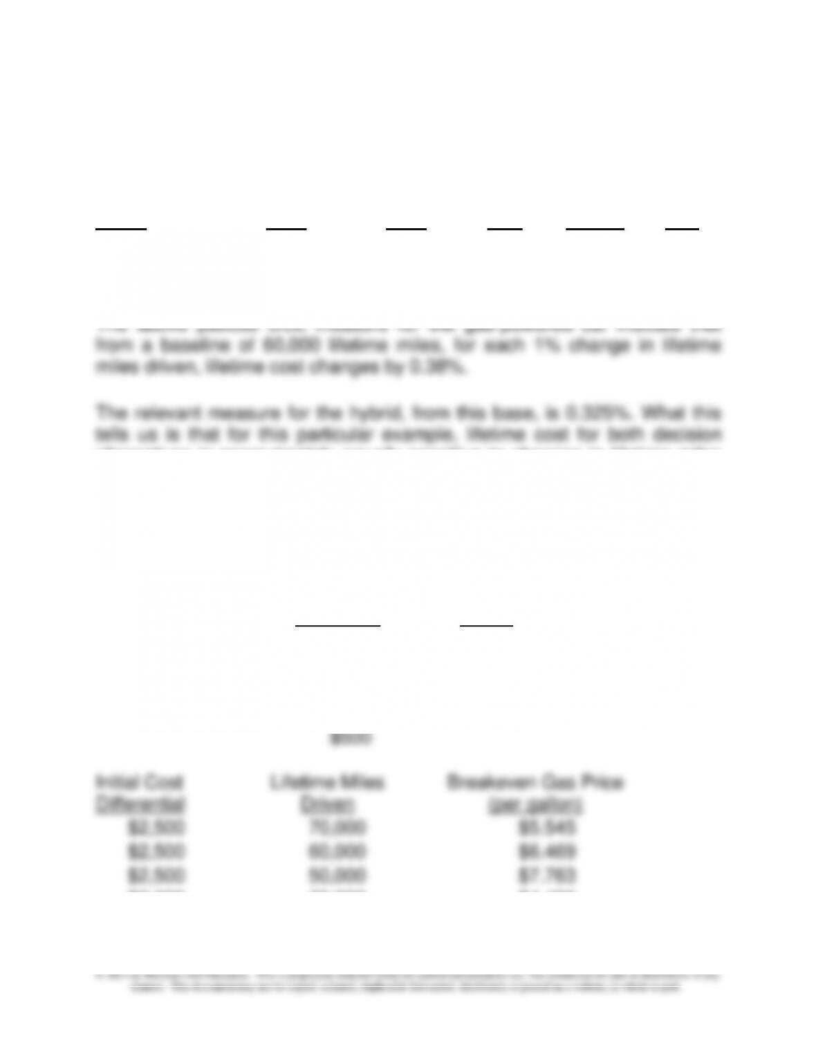
from a baseline of 60,000 lifetime miles, for each 1% change in lifetime
miles driven, lifetime cost changes by 0.38%.
The relevant measure for the hybrid, from this base, is 0.325%. What this
tells us is that for this particular example, lifetime cost for both decision
alternatives is approximately equally sensitive to changes in lifetime miles
driven.
5. Decision Table—Break-even gas price as a function of different
combinations of initial cost differential (Hybrid cost [net of rebate] −
Cost of gasoline-powered model) and lifetime miles driven
Initial Cost
Difference
Lifetime Miles
Driven
$2,500
70,000
$2,000
60,000
$1,500
50,000
$1,000
$500
Chapter 11 – Decision Making with a Strategic Emphasis
11–86
11–46 (continued-3)
Breakeven
Initial Cost Lifetime Miles Gas Price
Differential Driven (per gallon)
$1,500
70,000
$3.327
$1,500
60,000
$3.881
$1,500
50,000
$4.658
$1,000
70,000
$2.218
$1,000
60,000
$2.588
$1,000
50,000
$3.105
$500
70,000
$1.109
$500
60,000
$1.294
$500
50,000
$1.553
indifferent between the hybrid model and the gasoline-powered model.
Notice from the above table that the higher the initial cost differential for the
hybrid versus the gasoline-powered model, the greater the breakeven point
in terms of cost per gallon of fuel. You also notice that the breakeven gas
price is inversely related to lifetime miles driven. While both conclusions
seem intuitively appealing, the advantage of the decision table is the
structured way in which it allows you to deal quantitatively with uncertainty
surrounding the financial consequence of your decision choice.
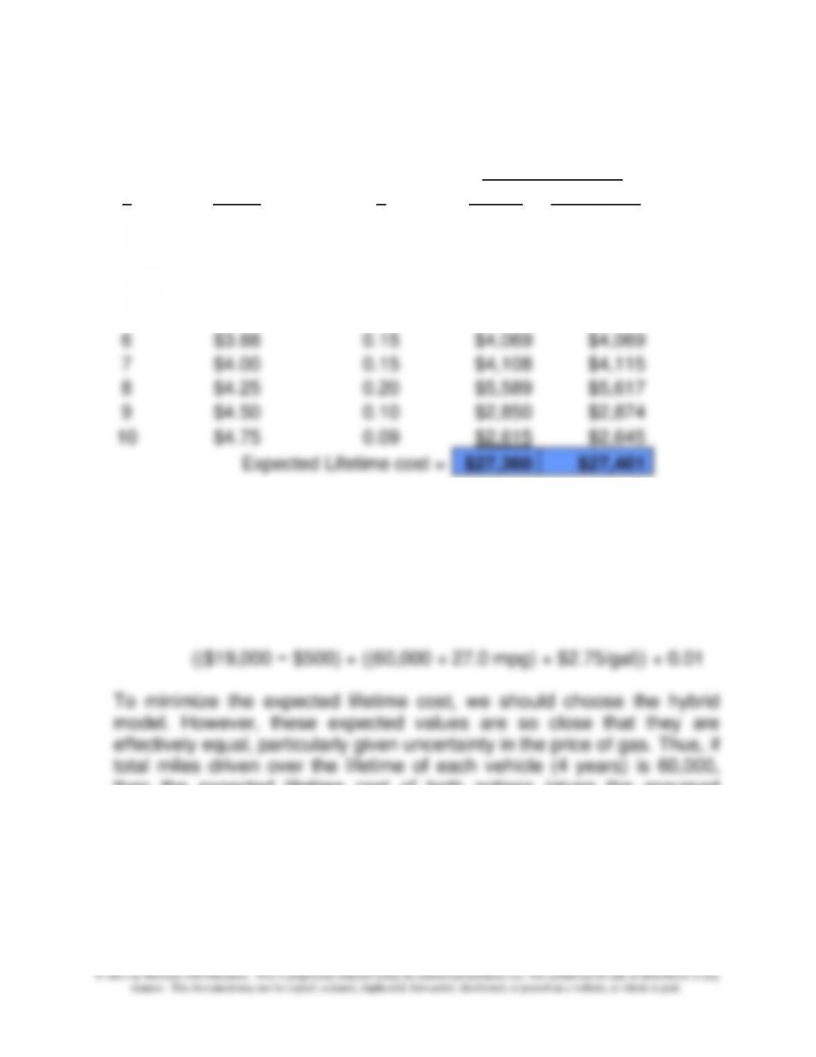
6. Expected value calculations:
10
E(ax) = ∑(Lifetime costi × pi)
i=1
$2,000
50,000
$6.210
Chapter 11 – Decision Making with a Strategic Emphasis
11–87
9-46 (continued-4)
Action (Decision)
i
Event
p
Hybrid
Gas Model
1
$2.75
0.01
$246
$242
2
$3.00
0.05
$1,258
$1,241
3
$3.25
0.05
$1,286
$1,274
4
$3.50
0.05
$1,314
$1,307
5
$3.75
0.15
$4,025
$4,017
6
$3.88
0.15
$4,069
$4,069
7
$4.00
0.15
$4,108
$4,115
8
$4.25
0.20
$5,589
$5,617
9
$4.50
0.10
$2,850
$2,874
10
$4.75
0.09
$2,615
$2,645
Expected Lifetime cost =
$27,360
$27,401
Lifetime cost = initial cost outlay (F) + variable (gas) cost over four-year
period
Example: for the hybrid model, if the probability of gas selling at
$2.75/gallon is 0.01, then the appropriate amount is cost
component for calculating expected lifetime cost is:
then the expected lifetime cost of both actions (given the assumed
probability distribution) is approximately equal.
Finally, note that basing the decision solely on expected value (in the
present case, cost) ignores the risk preferences (utility function) of the
decision-maker. The decision table presented above in part 5 can
facilitate this discussion.