Chapter 03 – Forecasting
3–41
Education.
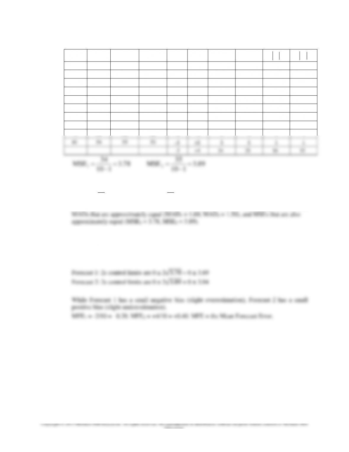
32. a.
Period
Actual
Forecast
1
Forecast
2
e1
e2
2
1
e
2
2
e
1
e
2
e
1
37
36
36
+1
+1
1
1
1
1
2
39
38
37
+1
+2
1
4
1
2
3
37
40
38
–3
–1
9
1
3
1
4
39
42
38
–3
+1
9
1
3
1
5
45
46
41
–1
+4
1
16
1
4
6
49
46
52
+3
–3
9
9
3
3
7
47
46
47
1
0
1
0
1
0
8
49
48
48
1
+1
1
1
1
1
9
51
52
52
–1
–1
1
1
1
1
10
54
55
53
–1
+1
1
1
1
1
–2
+4
34
35
16
15
50.1
10
15
MAD 60.1
10
16
MAD
89.3
110
35
MSE 78.3
110
34
MSE
21
21
The analyst is indifferent between the two alternatives because both forecasting methods have
b. The errors for Forecast 1 cycle (+1, +1, –3, –3, –1, +3, +1,+1, –1, –1), although all are within
2s control limits. The errors for Forecast 2 (+1, +2, –1, +1, +4, –3, 0, +1, –1, +1) do not
appear to cycle, but the error of +4 is just beyond the 2s control limits for Forecast 2.
Chapter 03 – Forecasting
3–42
Education.
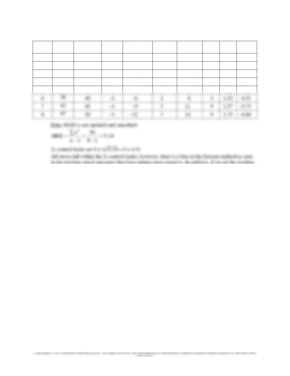
33.
t
Period
A
(Sales)
F
(Forecast)
A–F
(Error)
Cumulative
Error
Error
Error
Error2
MAD
TS
1
15
15
0
0
0
0
0
0.00
0.00
2
21
20
1
1
1
1
1
0.05
2.00
3
23
25
–2
–1
2
3
4
1.00
–1.00
4
30
30
0
–1
0
3
0
0.75
–1.33
5
32
35
–3
–4
3
6
9
1.20
–3.33
6
38
40
–2
–6
2
8
4
1.33
–4.51
7
42
45
–3
–9
3
11
9
1.57
–5.73
8
47
50
–3
–12
3
14
9
1.75
–6.86
Note: MAD is not updated and smoothed.
14.5
18
36
1
2
n
e
MSE
2s control limits are 0 ± 2√. = 0 ± 4.53
All errors fall within the 2s control limits; however, there is a bias in the forecast method as seen
in the tracking signal measures that keep getting more negative. In addition, if we set the tracking
signal limits at ± 4, then the tracking signals in periods 6 – 8 would fall outside the limits. In
conclusion, the forecast method is not performing adequately—it is exhibiting bias.
Chapter 03 – Forecasting
3–43
Education.
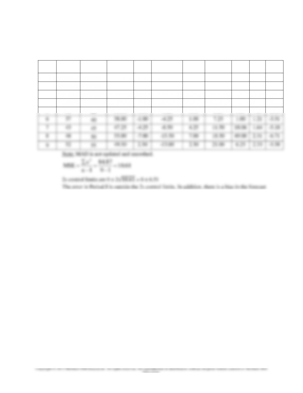
34.
t
Period
A
(sales)
T = 10 + 5t
T
F = T * S
Forecast
Error
Cumulative
Error
Error
Error
Error2
MAD
TS
1
14
15
13.50
0.50
0.50
0.50
0.50
0.25
0.50
1.00
2
20
20
19.00
1.00
1.50
1.00
1.50
1.00
0.75
2.00
3
24
25
26.25
-2.25
-0.75
2.25
3.75
5.06
1.25
-0.60
4
31
30
33.00
-2.00
-2.75
2.00
5.75
4.00
1.44
-1.91
5
31
35
31.50
-0.50
-3.25
0.50
6.25
0.25
1.25
-2.60
6
37
40
38.00
-1.00
-4.25
1.00
7.25
1.00
1.21
-3.51
7
43
45
47.25
-4.25
-8.50
4.25
11.50
18.06
1.64
-5.18
8
48
50
55.00
-7.00
-15.50
7.00
18.50
49.00
2.31
-6.71
9
52
55
49.50
2.50
-13.00
2.50
21.00
6.25
2.33
-5.58
Note: MAD is not updated and smoothed.
61.10
19
87.84
1
2
n
e
MSE
2s control limits are 0 ± 2√. = 0 ± 6.51
The error in Period 8 is outside the 2s control limits. In addition, there is a bias in the forecast
method as seen in the tracking signal measures that keep getting more negative (except in
Period 9). In addition, if we set the tracking signal limits at ± 4, then the tracking signals in
periods 7 – 9 would fall outside the limits. In conclusion, the forecast method is not
performing adequately. It is not in control and is exhibiting bias.
Chapter 03 – Forecasting
Case: M & L Manufacturing
1. The potential benefit of using a formalized approach to forecasting is that it will be easier to
utilize the computer and easier to quantify the information. A less formalized approach is more
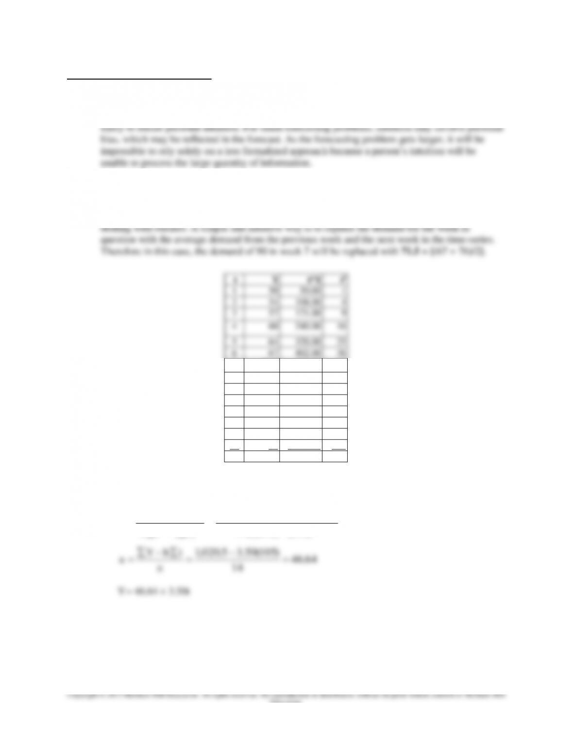
2. Product 1
Plotting the data for Product 1 reveals a linear pattern with the exception of demand in week 7.
Demand in week 7 is unusually high and does not fit the linear trend pattern of the remaining
data. Thus, the demand for the 7th week is considered an outlier. There are different ways of
Chapter 03 – Forecasting
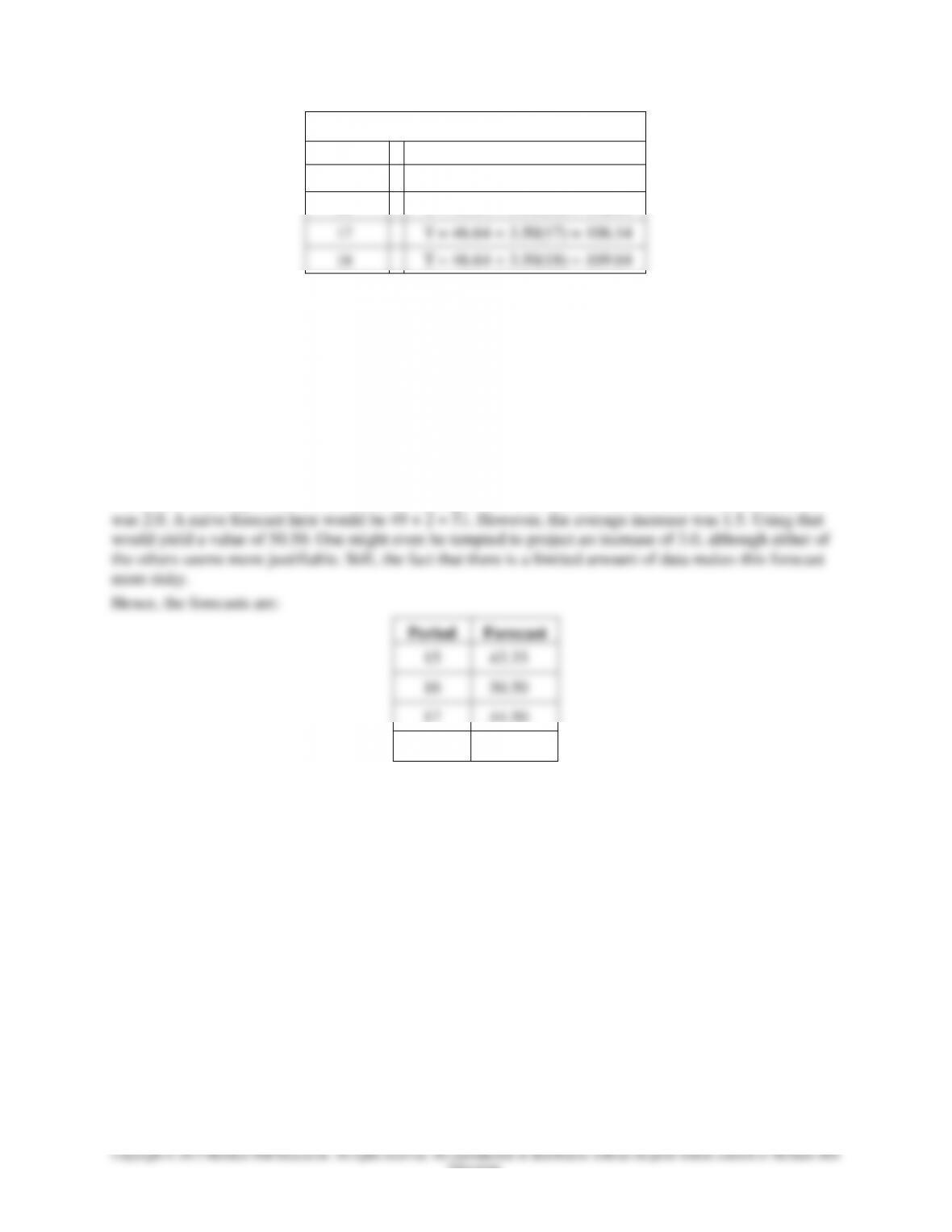
The next four forecasts (t = 15, 16, 17, 18) are:
Period
Forecast (T = 46.64 + 3.50t)
15
T = 46.64 + 3.50(15) = 99.14
16
T = 46.64 + 3.50(16) = 102.64
17
T = 46.64 + 3.50(17) = 106.14
18
T = 46.64 + 3.50(18) = 109.64
Product 2
Plotting the data for Product 2 yields a more complex pattern: There is a spike once every four weeks; the
values between the spikes are fairly close to each other. In addition, the data appear to be increasing at the
rate of about one unit per week. An intuitive approach would be to use the average of the three nonspike
periods plus 1.0 to predict the next three nonspike periods. Doing so for the data up to period 15 yields a
very small average forecast error (MAD = 0.54). Given the fact that we have only two data points
following the last spike, a reasonable forecast might be to use the last three period average plus 1.0 (i.e.,
43.33 to predict orders for period 15, and use the average of the values for periods 13 and 14 plus 1.0 (i.e.,
43.5 + 1.0 = 44.5) as a forecast for periods 17 and 18.
The values of the spikes also seem to be increasing. The initial increase was 1.0 and the second increase
Chapter 03 – Forecasting
Education.
Case: Highline Financial Services, Ltd.
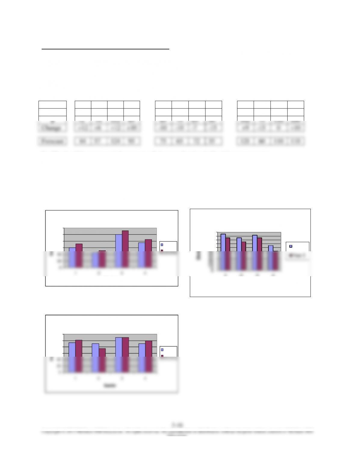
Aligning data by quarters, we can see (in the tables and in the figures) that demand for service A is
increasing, demand for service B is decreasing, and demand for service C is mixed. Note, though, that
total annual demand for service C has changed only slightly.
A Quarter B Quarter C Quarter
Year
1
2
3
4
1
2
3
4
1
2
3
4
1
60
45
100
75
95
85
92
65
93
90
110
90
2
72
51
112
85
85
75
85
50
102
75
110
100
Change
+12
+6
+12
+10
-10
-10
-7
-15
+9
-15
0
+10
Forecast
84
57
124
95
75
65
72
35
121
60
110
110
Freddie should be concerned about service B, because that has declined for every quarter.
Forecasts were made using a simple naïve (additive) approach. An argument could be made for using a
multiplicative approach (i.e., basing the forecast on the percentage change from one year to the next
instead of the actual change).
Service A
0
20
40
60
80
100
120
1 2 3 4
Quarter
Demand
Series1
Series2
0
10
20
30
40
50
60
70
80
90
100
1 2 3 4
Demand
Quarter
Service B
Year 1
Year 2
Service C
0
20
40
60
80
100
120
1 2 3 4
Quarter
Demand
Series1
Series2

Chapter 03 – Forecasting
Enrichment Module: Additional Methods for Evaluating Forecast Accuracy
The major problem in determining which forecast accuracy measure to use is that there is no universally
accepted accuracy measure. In Chapter 3, several different accuracy measures are covered. To develop a
better understanding of the forecast accuracy measures, first we must understand the nature of the forecast
errors. There are two types of forecast errors.
The first type of error is called the forecast bias, where the direction of the error is the primary
consideration. If the value of the error is negative, then we can conclude that the forecasting method
overestimated sales or demand. If the value of the error is positive, then we can conclude that the
forecasting method underestimated sales or demand because in calculating the error term, we always
subtract the forecasted value from the actual value. Below are three forecast accuracy measures to assess
forecast bias:
1. Mean Forecast Error (MFE)
2. Tracking Signal
3. Control Charts
When we sum the error terms, if there is no bias, positive and negative error terms will cancel each other
out, and the MFE will be zero. As was pointed out above, negative MFE is an indication of
overestimation, and positive MFE is an indication of underestimation. However, if the positive and
1. Mean Absolute Deviation (MAD)
2. Mean Squared Error (MSE)
3. Standard Error of Estimate
To be able to assess both the overall accuracy and forecast bias, an analyst probably should utilize at least