Chapter 19 – Linear Programming
19–61
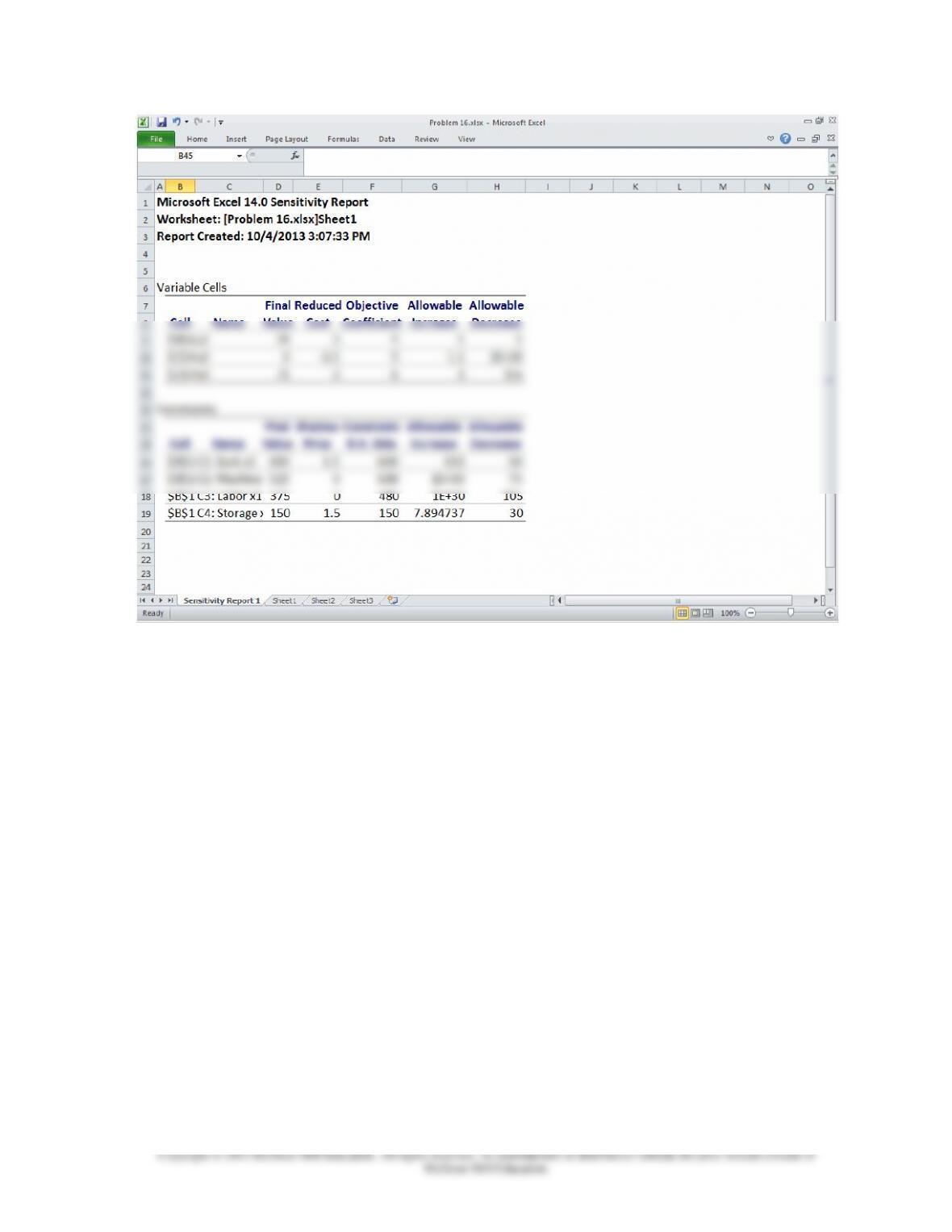
16. a. The marginal value (shadow price) of a pound of bark is $1.50 (refer to the Sensitivity
Report below for the Shadow Price of C1: Bark). This marginal value is in effect in the
range of feasibility: 600 – 50 to 600 + 150 = 550 lbs. to 750 lbs.
b. The maximum price the store would be justified in paying for additional bark is the
shadow price of $1.50 per pound.
c. The marginal value (shadow price) of labor is 0 because we currently have 105 excess
labor hours remaining (480 – 375). This marginal value is in effect in the range of
from $1,125 to $1,125 + (75 x $1) = $1,200.
g. To determine if the changes are within the range for multiple changes, refer to the
Sensitivity Report below and then compute the ratio of the amount of each change to the
end of the range in the same direction.
Chips (x3): Allowable Increase = $3 and proposed increase = $7 – $6 = $1.
Ratio = $1 / $3 = .333
Nuggets (x1): Allowable Decrease = $1 and proposed decrease = $.60.
Ratio = $.60 / $1.00 = .600.
The sum of the ratios = .333+ .600 = .933.
The sum of the ratios = .300 + .360 + .634 = 1.294.
Because the ratio > 1.00, we conclude that these changes do not fall within the range of
feasibility for multiple changes. Therefore, the LP model will need to be re-solved to
determine the impact.
Chapter 19 – Linear Programming
19–62
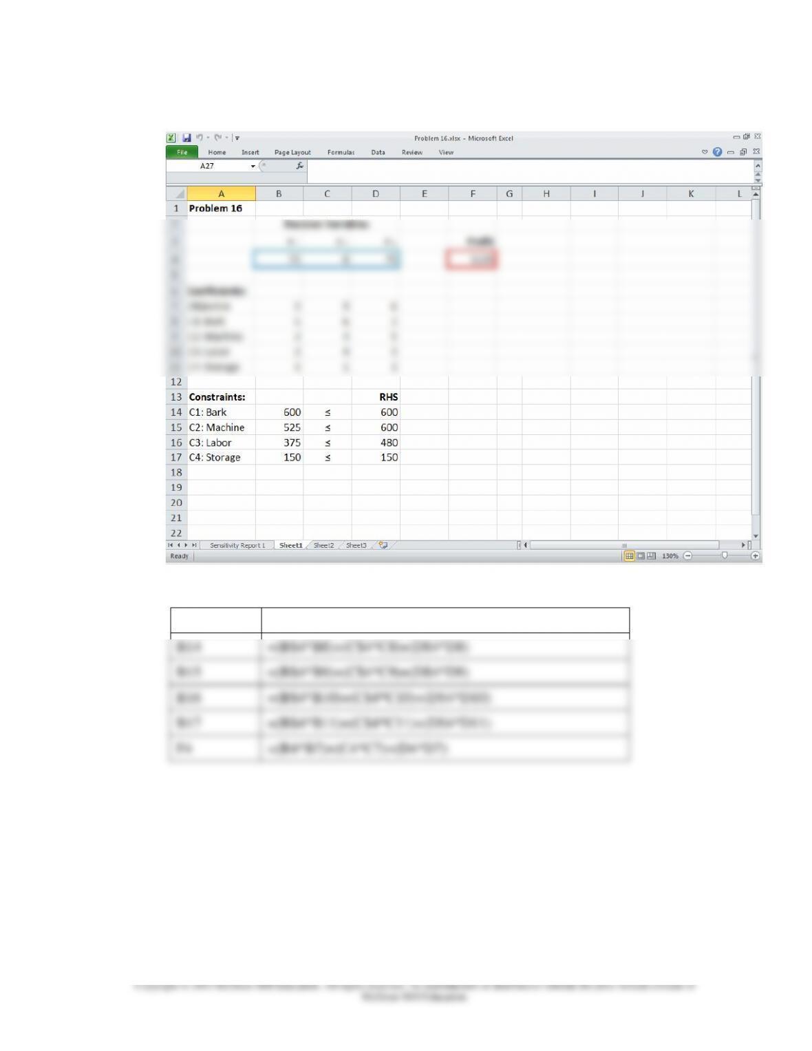
The Excel Solver solution and the Sensitivity Report are shown below:
Formulas used:
Cell
Formula
B14
=(B$4*B8)+(C$4*C8)+(D$4*D8)
B15
=(B$4*B9)+(C$4*C9)+(D$4*D9)
B16
=(B$4*B10)+(C$4*C10)+(D$4*D10)
B17
=(B$4*B11)+(C$4*C11)+(D$4*D11)
F4
=(B4*B7)+(C4*C7)+(D4*D7)
Chapter 19 – Linear Programming
19–63
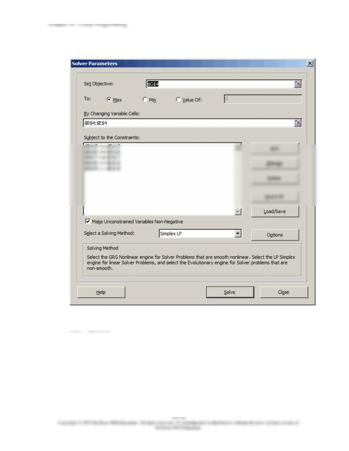
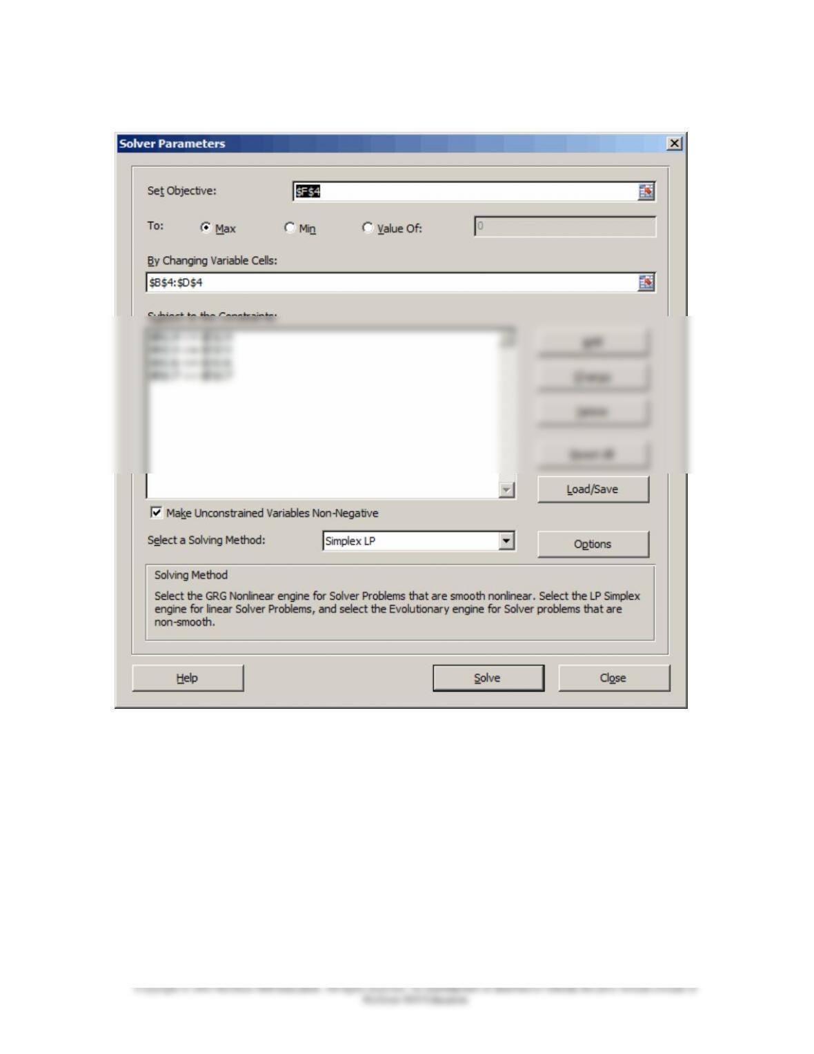
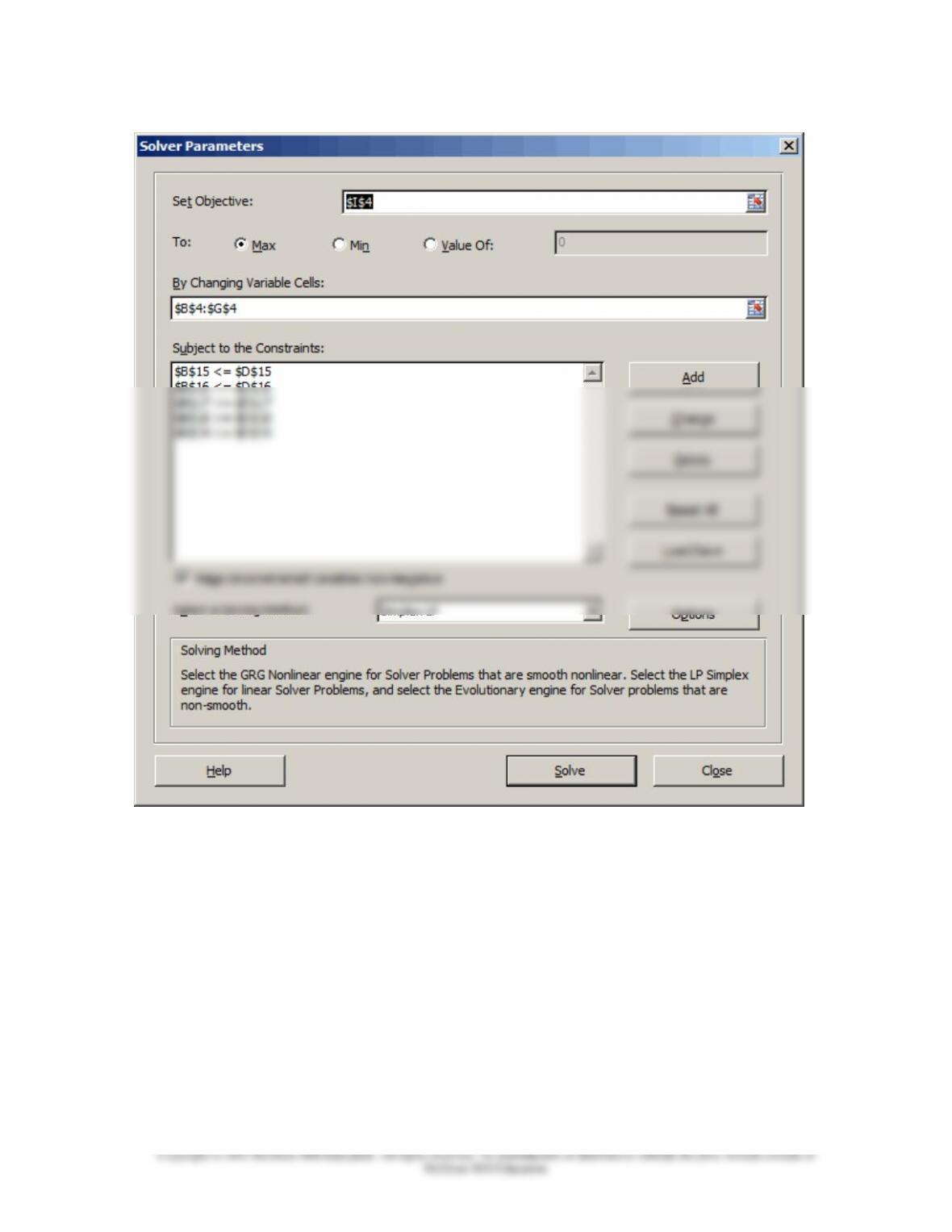
Solver Setup
Chapter 19 – Linear Programming
19–64
Chapter 19 – Linear Programming
19–65
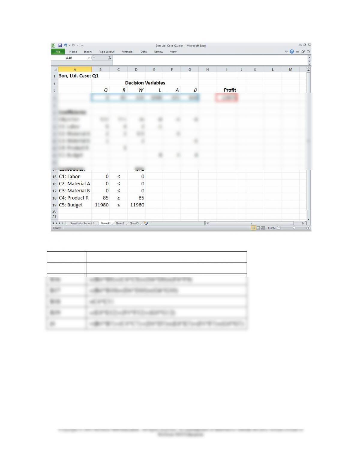
Solution to Son, Ltd. Case
Q = quantity of Product Q
L = quantity of labor
R = quantity of Product R
A = quantity of Material A
W = quantity of Product W
B = quantity of Material B
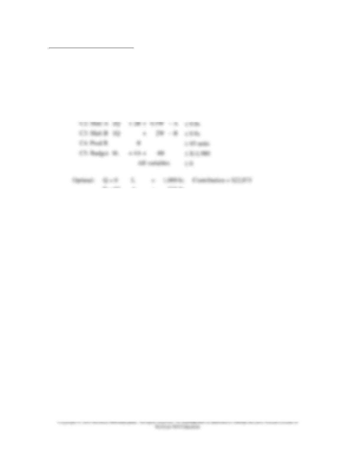
1. Maximize 122Q + 115R + 76W – 8L – 4A – 4B
Subject to:
C1: Labor
5Q
+ 4R
+
2W
– L
0 hr.
C2: Matl A
2Q
+ 2R
+
0.5W
– A
0 lb.
C3: Matl B
1Q
+
2W
– B
0 lb.
C4: Prod R
R
85 units
C5: Budget
8L
+ 4A
+
4B
$11,980
All variables
0
Optimal:
Q = 0
L =
1,000 hr.
Contribution = $22,875
R = 85
A =
335 lb.
W = 330
B =
660 lb.
The Excel Solver solution is shown below:
Chapter 19 – Linear Programming
19–66
Formulas used:
Cell
Formula
B15
=(B4*B8)+(C4*C8)+(D4*D8)+(E4*E8)
B16
=(B4*B9)+(C4*C9)+(D4*D9)+(F4*F9)
B17
=(B4*B10)+(D4*D10)+(G4*G10)
B18
=C4*C11
B19
=(E4*E12)+(F4*F12)+(G4*G12)
I4
=(B4*B7)+(C4*C7)+(D4*D7)+(E4*E7)+(F4*F7)+(G4*G7)
Chapter 19 – Linear Programming
19–67
Chapter 19 – Linear Programming
19–68
2. E = equal quantities of Q, R, and W
[E contribution per unit = 122 + 115 + 76 = 313]
[An alternate approach would be T = total amount, with an average contribution of 313/3 =
104.333]
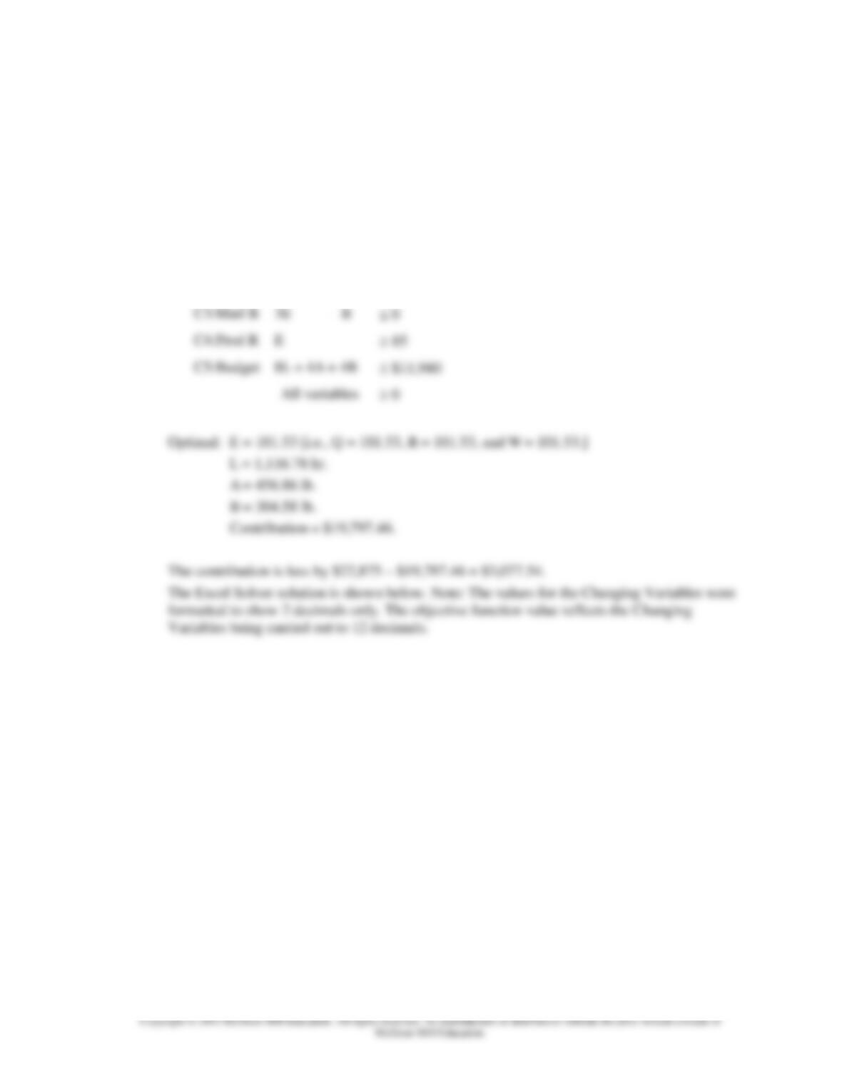
Maximize 313E – 8L – 4A – 4B
Subject to:
C1:Labor
11E
– L
0
C2:Matl A
4.5E
– A
0
C3:Matl B
3E
– B
0
C4:Prod R
E
85
C5:Budget
8L + 4A + 4B
$11,980
All variables
0
Optimal: E = 101.53 [i.e., Q = 101.53, R = 101.53, and W = 101.53.]
L = 1,116.78 hr.
A = 456.86 lb.
B = 304.58 lb.
Contribution = $19,797.46.
The contribution is less by $22,875 – $19,797.46 = $3,077.54.
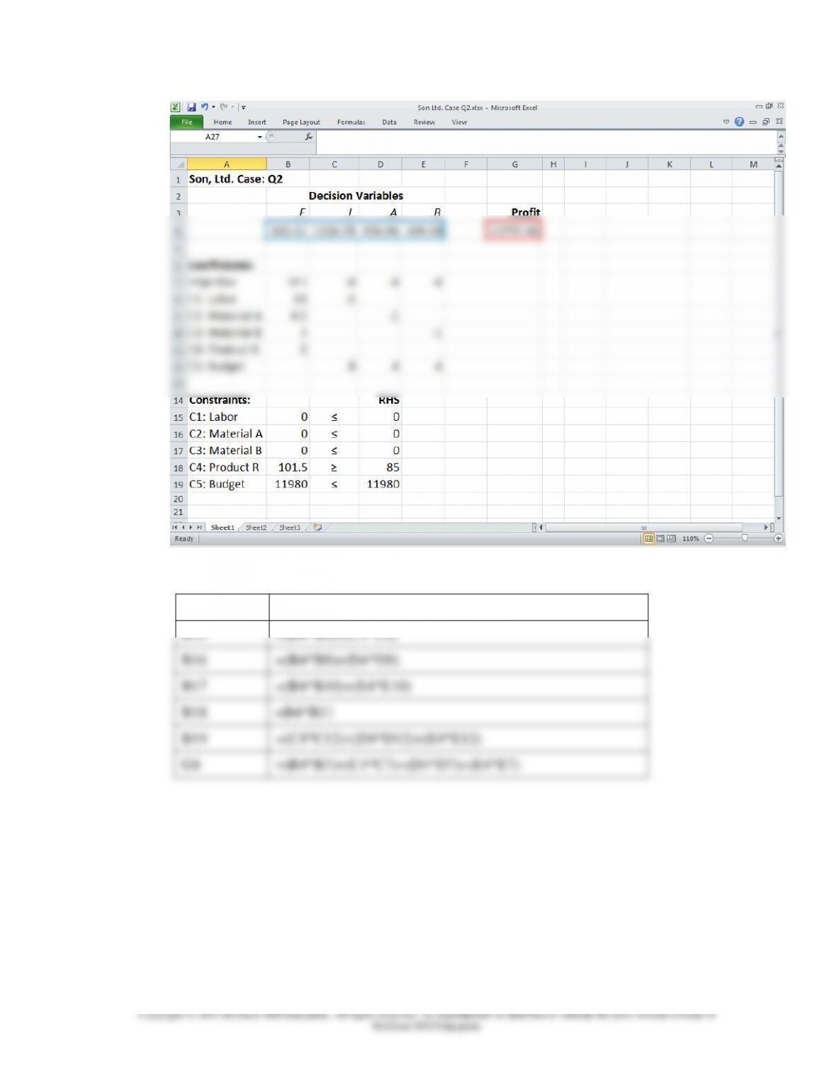
The Excel Solver solution is shown below. Note: The values for the Changing Variables were
formatted to show 2 decimals only. The objective function value reflects the Changing
Variables being carried out to 12 decimals.
Chapter 19 – Linear Programming
19–69
Formulas used:
Cell
Formula
B15
=(B4*B8)+(C4*C8)
B16
=(B4*B9)+(D4*D9)
B17
=(B4*B10)+(E4*E10)
B18
=B4*B11
B19
=(C4*C12)+(D4*D12)+(E4*E12)
G4
=(B4*B7)+(C4*C7)+(D4*D7)+(E4*E7)