
Chapter 06 – Accounting for Long-Term Operational Assets
6-1
General Comments for Chapter 6
Accounting for Long-Term Operational Assets
This chapter explains how acquiring, using, and disposing of long-term operational assets
affect financial statements. Because these activities span several accounting periods, we
recommend using a multicycle teaching model to illustrate accounting for them. Use a model
that presents financial statements vertically and accounting cycles horizontally. Students will see
how depreciation accumulates on the balance sheet and how cash flows occur in different periods
from expense recognition. You can visually portray the connections between asset usage and
revenue generation. The multicycle model is a powerful classroom learning tool.
The chapter covers basket purchases, alternative depreciation computations, revising
estimates and capital versus revenue expenditures, as well as depreciation, depletion, and
amortization. Considerable effort has been devoted to thinning the material into a manageable
set of concepts that all students will find useful. For example, the text omits the sum-of-the-
years’ digits method and partial period depreciation as well as depreciation for tax purposes.
Detailed Outline of a Lesson Plan for Chapter 6
I. Demonstration Problem 6-1 is based on a business that purchases an automobile
and then leases it to a customer. The problem illustrates three different depreciation
methods across four years.
A. Begin the problem by briefly discussing how to determine asset cost. The general
rule is that the cost of an asset includes any expenditure reasonably necessary to
obtain the asset and get it ready to use. With respect to Demonstration Problem 6-1
the automobile cost is $20,000 ($19,000 list − $1,000 cash discount + $2,000 interior
upgrade). The asset has a four-year useful life and a $4,000 salvage value.
B. Scenario 1. Explain that recognizing depreciation expense means allocating to
expense a portion of the cost of an operational asset. Next, have students calculate
depreciation expense for each of the four years using the straight-line method.
Briefly explain how depreciation is calculated using the straight-line method. When
most of the students have had ample time to work out the annual depreciation
expense, put the answer on the board so they can check their work. The annual
straight-line depreciation expense is $4,000 per year [($20,000 − $4,000) ÷ 4].
After they have determined the straight-line depreciation expense, have students
prepare financial statements for the first accounting cycle. You can save time by
using the work papers included in this manual. Computations for Scenario 1
(straight-line depreciation) are shown below:
Year 2014
1. Revenue. The problem specifies the 2014 revenue, $7,200.
6-3
C. Scenario 2. Before proceeding to Scenario 2 you will need to show your students
how to compute double-declining-balance depreciation. The computations are shown
below for your convenience:
Year
(Cost
─
Accumulated
Depreciation)
x
(2 x Straight-
Line Rate)
=
Depreciation
Expense
2014
(20,000
─
$ -0-)
x
.5
=
$10,000
2015
(20,000
─
10,000)
x
.5
=
5,000
2016
(20,000
─
15,000)
x
.5
=
1,000*
2017
(20,000
─
16,000)
x
.5
=
0*
*The 2016 formula yields $2,500. However, only $1,000 can be charged
because the asset cannot be depreciated below its salvage value.
Similarly, the amount of depreciation recognized in 2017 is zero because
the asset has been fully depreciated.
After you have shown students how to compute depreciation expense, have them
complete the financial statements. Again, using the work papers will save class time.
We suggest you help the students get started by working through the 2014 statements
step by step. The logic for determining the amounts on the statements is described
above in the explanation for Scenario 1. Although amounts for some items differ, the
logic is the same.
Once the students have completed the financial statements, it is a good idea to
have them compare Scenario 2 statements with Scenario 1 statements. Point out that
the end result is the same under either method. The difference lies in the timing
rather than the total amount of expense recognized. Point out that the scenarios
involve different amounts of revenue recognition and cash flow each year (although
the same amounts for the term of the lease as a whole).
D. Scenario 3. Before proceeding to Scenario 3 you will need to show your students
how to compute units-of-production depreciation. The computations are shown
below for your convenience:
Begin by determining the depreciation cost per mile:
(Cost − Salvage Value) ÷ Number of Miles = Depreciation Cost Per Mile
($20,000 − $4,000) ÷ 100,000 = $0.16 per mile
Determine the annual depreciation expense by multiplying the number of miles
driven during the year by the depreciation cost per mile.
Year
Miles Driven
x
Cost Per Mile
=
Depreciation Expense
2014
30,000
x
0.16
=
$4,800
2015
10,000
x
0.16
=
1,600
2016
40,000
x
0.16
=
6,400
2017
25,000
x
0.16
=
3,200*

Chapter 06 – Accounting for Long-Term Operational Assets
6-4
*The 2017 formula yields $4,000. However, only $3,200 can
be charged because the asset cannot be depreciated below its
salvage value.
After you have shown students how to compute depreciation expense, have them
complete the financial statements. Again, help them get started by working through
the 2014 statements step by step. The logic for determining the amounts on the
statements is described above in the explanation for Scenario 1. Although amounts
for some items differ, the logic is the same. Students are likely to need less help for
this scenario than they needed before.
Once the students have completed the financial statements, it is a good idea to
have them compare the financial statements generated under all three scenarios.
Emphasize that the end result is the same regardless of depreciation method. The
difference lies in the timing rather than the total amount of expense recognized.
II. Demonstration Problem 6-2 introduces accounting for capital expenditures and
maintenance costs incurred after the acquisition date. The objectives are twofold: to
illustrate how maintenance costs affect the financial statements differently than capital
expenditures; and to show how capital expenditures made to improve the quality of an
asset differ from those made to extend the useful life of the asset. The statements model
is suited to these instructional objectives. Draw or display a statements model. Then
show students how maintenance costs and capital expenditures affect financial statements
differently.
III. Introduce accounting for natural resources. Highlight the similarities between units-
of-production depreciation and depletion. Use Exercise 6-18 as a demonstration
problem.
IV. Introduce accounting for intangible assets. Highlight the similarities between straight-
line depreciation and amortization computations. Use Exercise 6-19 as a demonstration
problem.
V. Time considerations and homework assignments. Plan to spend approximately one
hour of class time on the different depreciation methods. Allow an additional hour to
cover related subjects such as basket purchases and accounting for capital expenditures,
depletion, and amortization of intangibles. Problem 6-28 is a multicycle problem that
will allow students to see how depreciation affects financial statements over an asset’s
life cycle. Problem 6-23 requires applying different depreciation methods to the same
asset. Students will see that the amount of expense recognized in any single accounting
period is affected by the type of depreciation method chosen. Exercise 6-17 involves
capital expenditures. Problem 6-30 covers depletion. Problems 6-32 and 6-33 address
intangible assets.
Chapter 06 – Accounting for Long-Term Operational Assets
6-5
Demonstration Problems for Chapter 6
Demonstration Problem 6-1: Alternative Depreciation Methods
The following events pertain to Sanders Rental Company (SRC).
1. SRC was started when it issued common stock for $21,000 cash.
2. On January 1, 2014, SRC paid cash to purchase an automobile. The car dealer gave SRC a
$1,000 cash discount off the $19,000 list price. However, SRC paid an additional $2,000 to
equip the car with a more luxurious interior so it would have greater appeal to its clientele.
Sanders Rental Company expected the car to have a four-year useful life and a $4,000
salvage value. SRC expected to lease the car for 100,000 miles before disposing of it.
3. SRC leased the car to a customer who drove it 30,000 / 10,000 / 40,000 / 25,000 miles
during 2014, 2015, 2016, and 2017, respectively. SRC sold the car on January 1, 2018, for
$4,300 cash.
4. Assume SRC recognized depreciation expense using one of three separate scenarios. The
revenue stream and amounts of cash flows assumed for each scenario are shown below:
Revenue Stream
Scenario
2014
2015
2016
2017
1
$ 7,200
$7,200
$7,200
$7,200
2
$13,200
$8,200
$4,200
$3,200
3
$ 8,000
$4,800
$9,600
$6,400
Use the following depreciation method for each of the scenarios.
Scenario
Depreciation Method
1
Straight-Line
2
Double-Declining-Balance
3
Units-of-Production
Required
Prepare income statements, balance sheets, and statements of cash flows for 2014 through 2017
for each of the three scenarios.
Chapter 06 – Accounting for Long-Term Operational Assets
6-6
Education.
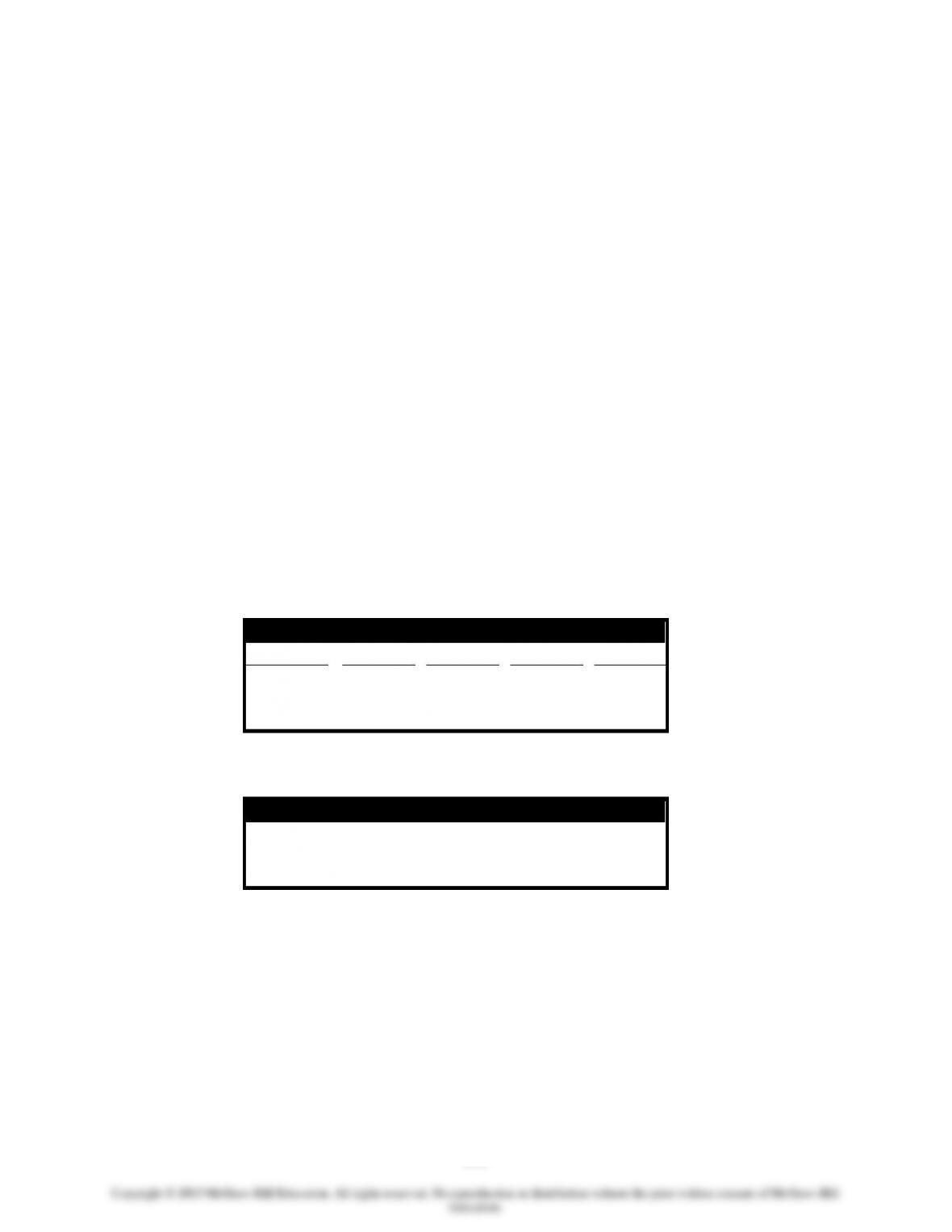
Demonstration Problem 6-2: Capital vs. Revenue Expenditures
The following statements model depicts the financial condition of Boston Mechanical Company
just prior to an expenditure of $1,000 cash.
Assets
=
Liab.
+
Equity
Rev.
–
Exp.
=
Net Inc.
Cash Flow
Cash
+
Equip.
+
Accum.
Dep.
=
Ret. Ear.
1,000
+
5,000
−
(2,000)
=
-0-
+
4,000
-0-
–
-0-
=
-0-
-0-
Required
Show the effects of the expenditure on the statements model under the following three separate
scenarios.
1. The $1,000 was paid for routine maintenance cost.
2. The $1,000 was paid to improve the quality of the equipment.
3. The $1,000 was paid to extend the useful life of the equipment.
SOLUTIONS TO
DEMONSTRATION PROBLEM
Demonstration Problem 6-1: Solution, Scenario 1
Straight-Line Depreciation
Income Statements
2014
2015
2016
2017
2018
Rent Revenue
$7,200
$7,200
$7,200
$7,200
$ -0-
Depreciation Expense
4,000
4,000
4,000
4,000
-0-
Operating Income
$3,200
$3,200
$3,200
$3,200
$ -0-
Gain on Sale
of Automobile
-0-
-0-
-0-
-0-
$ 300
Net Income
$3,200
$3,200
$3,200
$3,200
$ 300
Balance Sheets
Assets
Cash
$ 8,200
$15,400
$22,600
$29,800
$34,100
Automobile
20,000
20,000
20,000
20,000
-0-
Accumulated Dep.
(4,000)
(8,000)
(12,000)
(16,000)
-0-
Total Assets
$24,200
$27,400
$30,600
$33,800
$34,100
Stockholders’ Equity
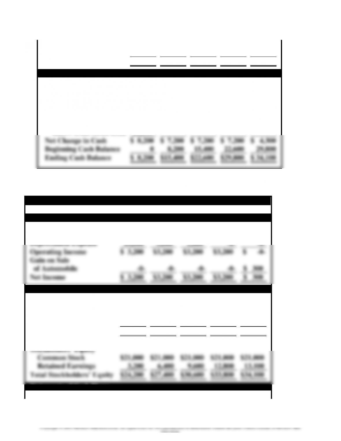
Chapter 06 – Accounting for Long-Term Operational Assets
6-7
Education.
Common Stock
$21,000
$21,000
$21,000
$21,000
$21,000
Retained Earnings
3,200
6,400
9,600
12,800
13,100
Total Stockholders’ Equity
$24,200
$27,400
$30,600
$33,800
$34,100
Statements of Cash Flows
Operating Activities
Inflow from Customer
$ 7,200
$ 7,200
$ 7,200
$ 7,200
$ -0-
Investing Activities
Outflow for Automobile
(20,000)
Inflow from Sale of Auto
4,300
Financing Activities
Inflow from Stock Issue
21,000
Net Change in Cash
$ 8,200
$ 7,200
$ 7,200
$ 7,200
$ 4,300
Beginning Cash Balance
0
8,200
15,400
22,600
29,800
Ending Cash Balance
$ 8,200
$15,400
$22,600
$29,800
$ 34,100
Demonstration Problem 6-1: Solution, Scenario 2
Double-Declining-Balance Depreciation
Income Statements
2014
2015
2016
2017
2018
Rent Revenue
$13,200
$8,200
$4,200
$3,200
$ -0-
Depreciation Expense
10,000
5,000
1,000
-0-
-0-
Operating Income
$ 3,200
$3,200
$3,200
$3,200
$ -0-
Gain on Sale
of Automobile
-0-
-0-
-0-
-0-
$ 300
Net Income
$ 3,200
$3,200
$3,200
$3,200
$ 300
Balance Sheets
Assets
Cash
$14,200
$22,400
$26,600
$29,800
$34,100
Automobile
20,000
20,000
20,000
20,000
-0-
Accumulated Dep.
(10,000)
(15,000)
(16,000)
(16,000)
-0-
Total Assets
$24,200
$27,400
$30,600
$33,800
$34,100
Stockholders’ Equity
Common Stock
$21,000
$21,000
$21,000
$21,000
$21,000
Retained Earnings
3,200
6,400
9,600
12,800
13,100
Total Stockholders’ Equity
$24,200
$27,400
$30,600
$33,800
$34,100
Statements of Cash Flows
Operating Activities
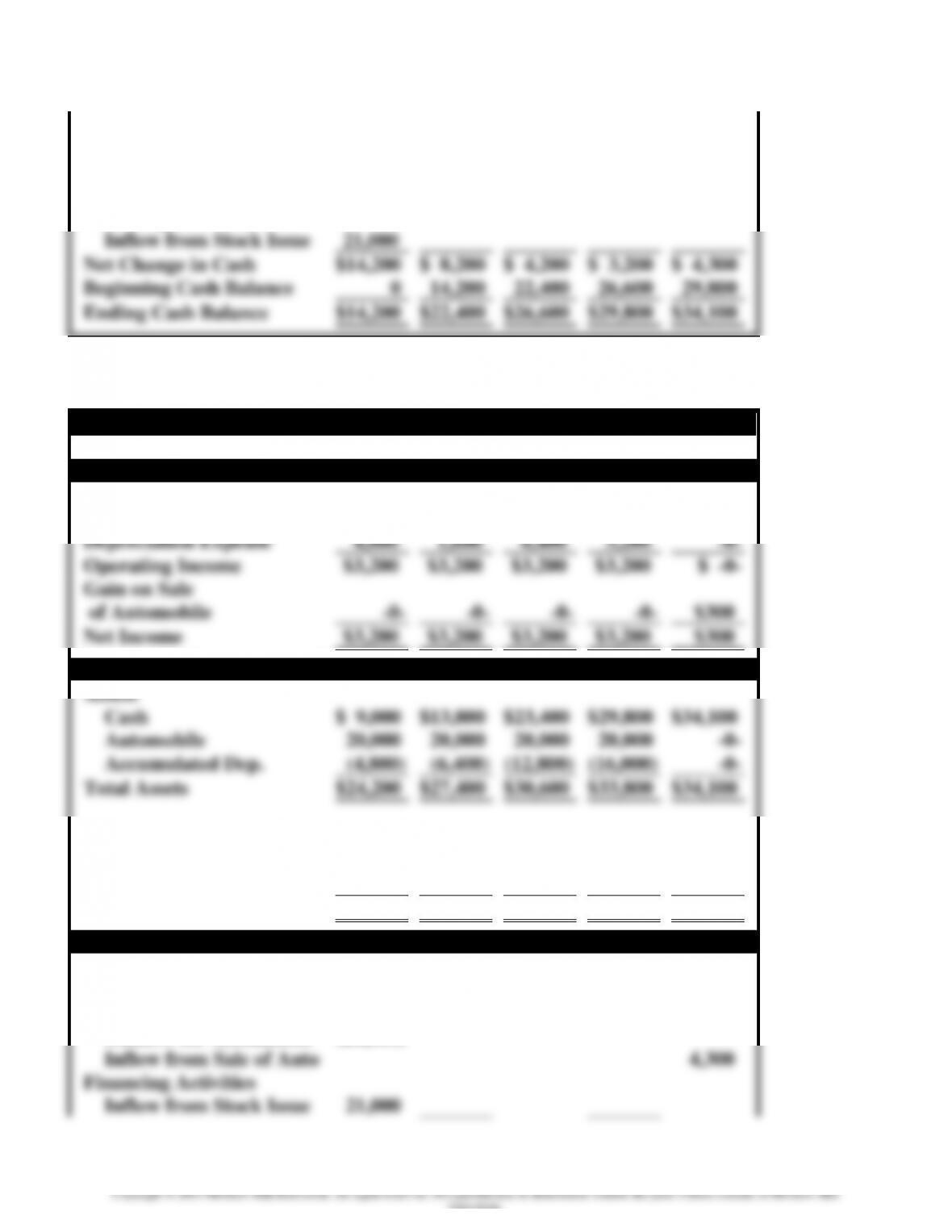
Chapter 06 – Accounting for Long-Term Operational Assets
6-8
Education.
Inflow from Customer
$13,200
$8,200
$4,200
$3,200
$ -0-
Investing Activities
Outflow for Automobile
(20,000)
Inflow from Sale of Auto
4,300
Financing Activities
Inflow from Stock Issue
21,000
Net Change in Cash
$14,200
$ 8,200
$ 4,200
$ 3,200
$ 4,300
Beginning Cash Balance
0
14,200
22,400
26,600
29,800
Ending Cash Balance
$14,200
$22,400
$26,600
$29,800
$34,100
Demonstration Problem 6-1: Solution, Scenario 3
Units-of-Production Depreciation
Income Statements
2014
2015
2016
2017
2018
Rent Revenue
$8,000
$4,800
$9,600
$6,400
$ -0-
Depreciation Expense
4,800
1,600
6,400
3,200
-0-
Operating Income
$3,200
$3,200
$3,200
$3,200
$ -0-
Gain on Sale
of Automobile
-0-
-0-
-0-
-0-
$300
Net Income
$3,200
$3,200
$3,200
$3,200
$300
Balance Sheets
Assets
Cash
$ 9,000
$13,800
$23,400
$29,800
$34,100
Automobile
20,000
20,000
20,000
20,000
-0-
Accumulated Dep.
(4,800)
(6,400)
(12,800)
(16,000)
-0-
Total Assets
$24,200
$27,400
$30,600
$33,800
$34,100
Stockholders’ Equity
Common Stock
$21,000
$21,000
$21,000
$21,000
$21,000
Retained Earnings
3,200
6,400
9,600
12,800
13,100
Total Stockholders’ Equity
$24,200
$27,400
$30,600
$33,800
$34,100
Statements of Cash Flows
Operating Activities
Inflow from Customer
$ 8,000
$ 4,800
$ 9,600
$ 6,400
$ -0-
Investing Activities
Outflow for Automobile
(20,000)
Inflow from Sale of Auto
4,300
Financing Activities
Inflow from Stock Issue
21,000
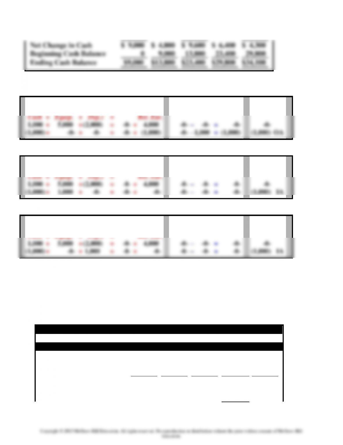
Chapter 06 – Accounting for Long-Term Operational Assets
6-9
Net Change in Cash
$ 9,000
$ 4,800
$ 9,600
$ 6,400
$ 4,300
Beginning Cash Balance
0
9,000
13,800
23,400
29,800
Ending Cash Balance
$9,000
$13,800
$23,400
$29,800
$34,100
Demonstration Problem 6-2: Solution
1. Paid $1,000 cash for routine maintenance cost.
Assets
=
Liab.
+
Equity
Rev.
–
Exp.
=
Net Inc.
Cash Flow
Cash
+
Equip.
+
(Accum.
Dep.)
=
Ret. Ear.
1,000
+
5,000
+
(2,000)
=
-0-
+
4,000
-0-
–
-0-
=
-0-
-0-
(1,000)
+
-0-
+
-0-
=
-0-
+
(1,000)
-0-
–
1,000
=
(1,000)
(1,000) OA
2. Paid $1,000 cash to improve the quality of the equipment.
Assets
=
Liab.
+
Equity
Rev.
–
Exp.
=
Net Inc.
Cash Flow
Cash
+
Equip.
+
(Accum.
Dep.)
=
Ret. Ear.
1,000
+
5,000
+
(2,000)
=
-0-
+
4,000
-0-
–
-0-
=
-0-
-0-
(1,000)
+
1,000
+
-0-
=
-0-
+
-0-
-0-
–
-0-
=
-0-
(1,000) IA
3. Paid $1,000 cash to extend the useful life of the equipment.
Assets
=
Liab.
+
Equity
Rev.
–
Exp.
=
Net Inc.
Cash Flow
Cash
+
Equip.
+
(Accum.
Dep.)
=
Ret. Ear.
1,000
+
5,000
+
(2,000)
=
-0-
+
4,000
-0-
–
-0-
=
-0-
-0-
(1,000)
+
-0-
+
1,000
=
-0-
+
-0-
-0-
–
-0-
=
-0-
(1,000) IA
WORK PAPERS FOR
DEMONSTRATION PROBLEMS
Demonstration Problem 6-1: Work Paper, Scenario 1
Straight-Line Depreciation
Income Statements
2014
2015
2016
2017
2018
Rent Revenue
$7,200
$7,200
$7,200
$7,200
$ -0-
Depreciation Expense
Operating Income
Gain on Sale
of Automobile
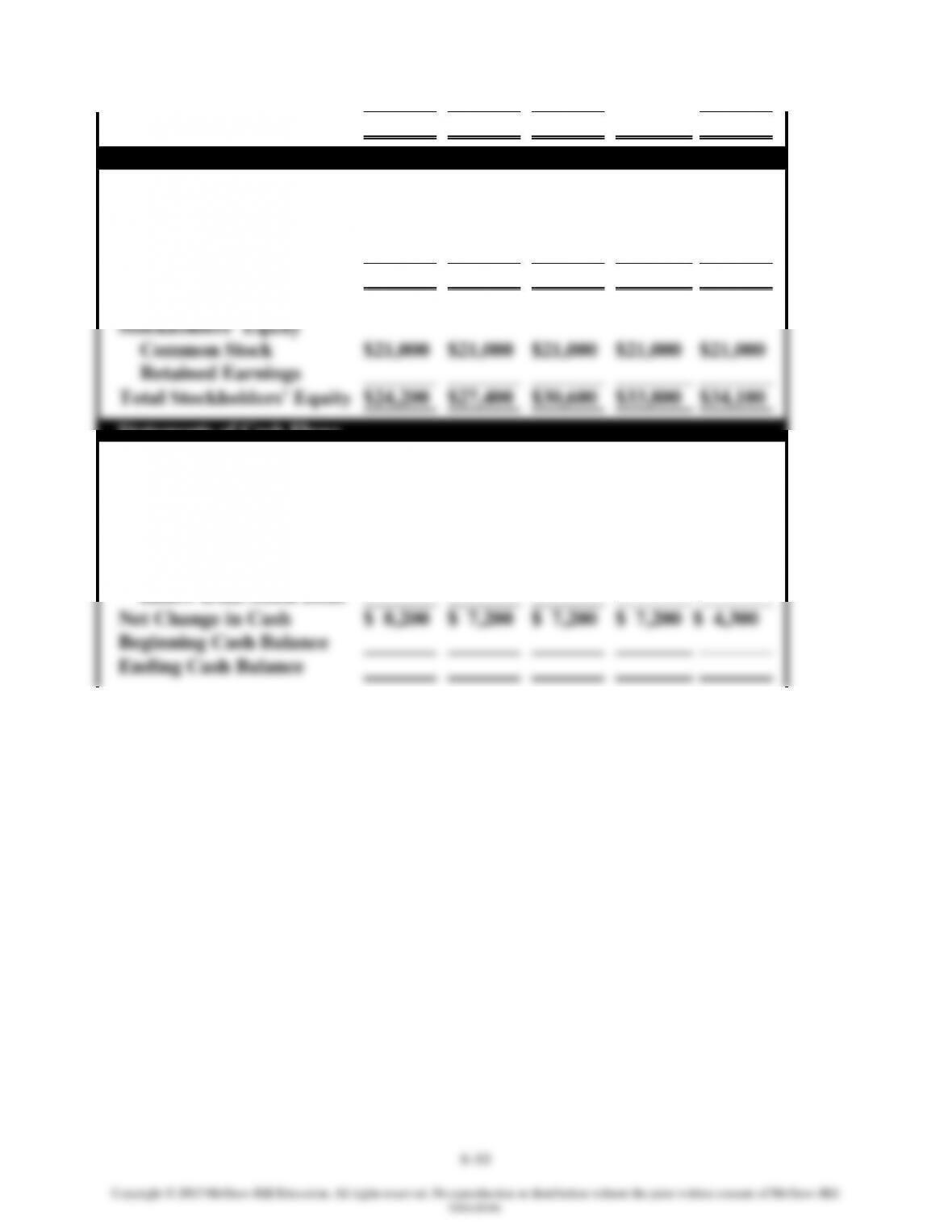
Chapter 06 – Accounting for Long-Term Operational Assets
Net Income
$ 300
Balance Sheets
Assets
Cash
Automobile
Accumulated Dep.
Total Assets
Stockholders’ Equity
Common Stock
$21,000
$21,000
$21,000
$21,000
$21,000
Retained Earnings
Total Stockholders’ Equity
$24,200
$27,400
$30,600
$33,800
$34,100
Statements of Cash Flows
Operating Activities
Inflow from Customer
Investing Activities
Outflow for Automobile
Inflow from Sale of Auto
Financing Activities
Inflow from Stock Issue
Net Change in Cash
$ 8,200
$ 7,200
$ 7,200
$ 7,200
$ 4,300
Beginning Cash Balance
Ending Cash Balance