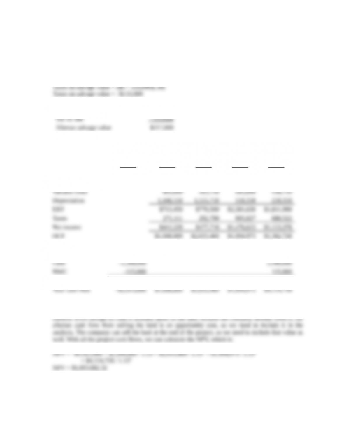
31. We will begin by calculating the aftertax salvage value of the equipment at the end of the project’s
life. The aftertax salvage value is the market value of the equipment minus any taxes paid (or
refunded), so the aftertax salvage value in four years will be:
Taxes on salvage value = (BV – MV)TC
Market price $350,000
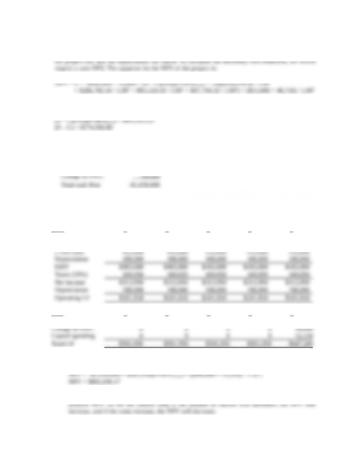
Now we need to calculate the operating cash flow each year. Using the bottom up approach to
calculating operating cash flow, we find:
Year 0 Year 1 Year 2 Year 3 Year 4
Revenues $2,700,000 $3,225,000 $3,900,000 $2,925,000
Fixed costs 415,000 415,000 415,000 415,000
Capital spending –$3,500,000 $217,000
Notice the calculation of the cash flow at Time 0. The capital spending on equipment and investment
in net working capital are both cash outflows. The aftertax selling price of the land is also a cash
The company should accept the new product line.
CHAPTER 10 – 2
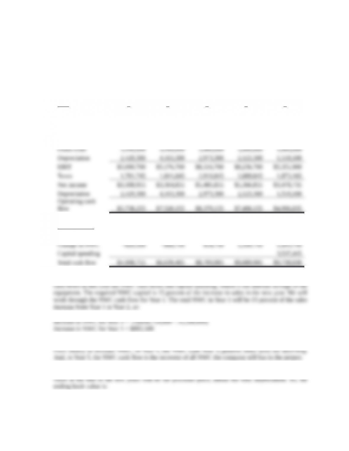
32. This is an in-depth capital budgeting problem. Probably the easiest OCF calculation for this problem
is the bottom up approach, so we will construct an income statement for each year. Beginning with
the initial cash flow at time zero, the project will require an investment in equipment. The project
will also require an investment in NWC. The initial NWC investment is given, and the subsequent
NWC investment will be 15 percent of the increase in the following year’s sales. So, the cash flow
required for the project today will be:
Capital spending –$17,000,000
CHAPTER 10 – 3
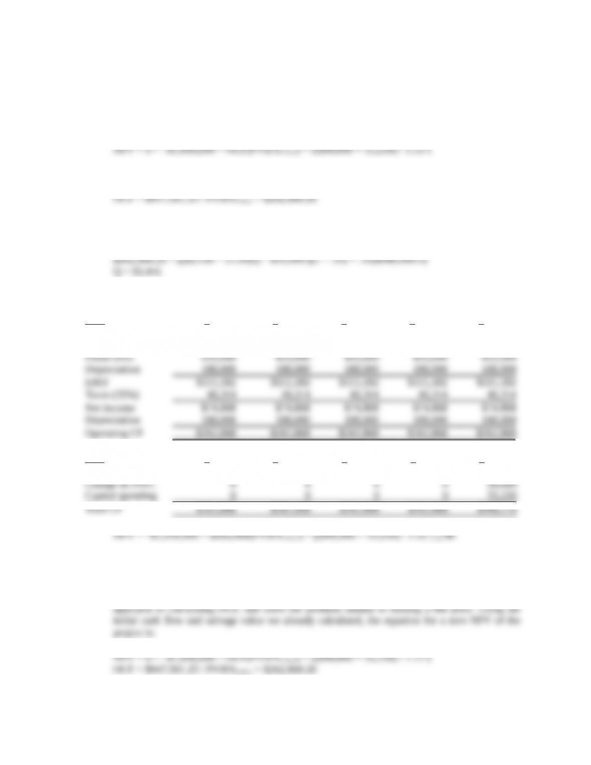
Now we can begin the remaining calculations. Sales figures are given for each year, along with the
price per unit. The variable costs per unit are used to calculate total variable costs, and fixed costs
are given at $1,500,000 per year. To calculate depreciation each year, we use the initial equipment
cost of $17 million, times the appropriate MACRS depreciation each year. The remainder of each
income statement is calculated below. Notice at the bottom of the income statement we added back
depreciation to get the OCF for each year. The section labeled “Net cash flows” will be discussed
below:
Year 1 2 3 4 5
Ending book value $14,570,700 $10,407,400 $7,434,100 $5,310,800 $3,792,700
Sales $33,180,000 $38,710,000 $44,635,000 $41,870,000 $31,205,000
Variable costs 22,260,000 25,970,000 29,945,000 28,090,000 20,935,000
Net cash flows
Operating CF $5,738,255 $7,528,155 $8,379,155 $7,490,155 $4,996,835
After we calculate the OCF for each year, we need to account for any other cash flows. The other
Notice that the NWC cash flow is negative. Since the sales are increasing, we will have to spend
To calculate the aftertax salvage value, we first need the book value of the equipment. The book
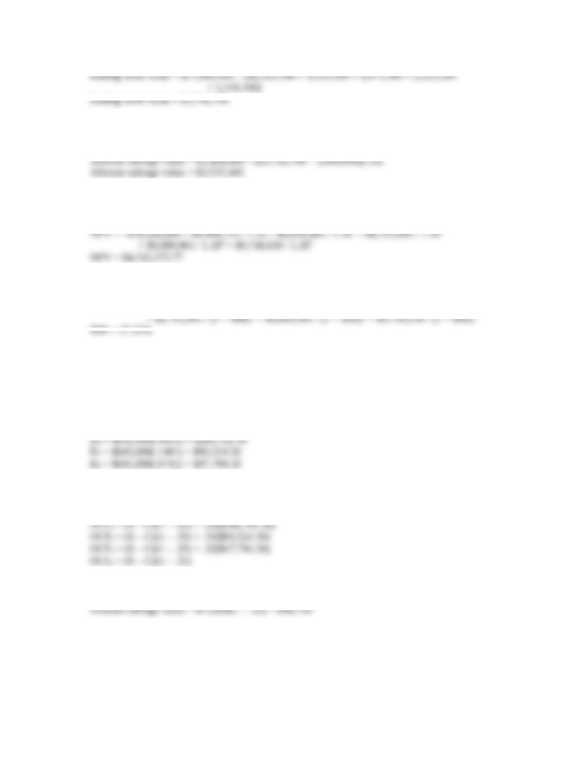
CHAPTER 10 – 4
The market value of the used equipment is 20 percent of the purchase price, or $3.4 million, so the
aftertax salvage value will be:
The aftertax salvage value is included in the total cash flows as capital spending. Now we have all of
the cash flows for the project. The NPV of the project is:
And the IRR is:
NPV = 0 = –$18,500,000 + $4,908,755 / (1 + IRR) + $6,639,405 / (1 + IRR)2
We should accept the project.
33. To find the initial pretax cost savings necessary to buy the new machine, we should use the tax shield
approach to find the OCF. We begin by calculating the depreciation each year using the MACRS
depreciation schedule. The depreciation each year is:
D1 = $645,000(.3333) = $214,978.50
Using the tax shield approach, the OCF each year is:
OCF1 = (S – C)(1 – .35) + .35($214,978.50)
Now we need the aftertax salvage value of the equipment. The aftertax salvage value is:
CHAPTER 10 – 5
To find the necessary cost reduction, we must realize that we can split the cash flows each year. The OCF
in any given year is the cost reduction (S – C) times one minus the tax rate, which is an annuity for
Solving this equation for the sales minus costs, we get:
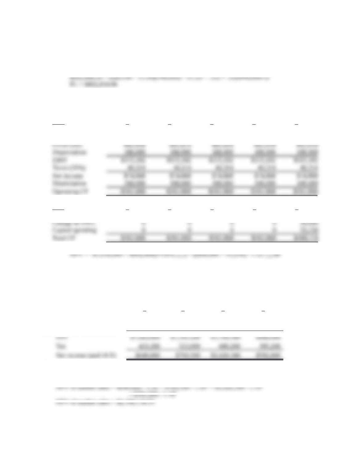
34. a. This problem is basically the same as Problem 18, except we are given a sales price. The cash
flow at Time 0 for all three parts of this question will be:
Capital spending –$940,000
We will use the initial cash flow and the salvage value we already found in that problem. Using
the bottom-up approach to calculating the OCF, we get:
Assume price per unit = $23 and units/year = 140,000
Year 1 2 3 4 5
Sales $3,220,000 $3,220,000 $3,220,000 $3,220,000 $3,220,000
Variable costs 2,114,000 2,114,000 2,114,000 2,114,000 2,114,000
Year 1 2 3 4 5
Operating CF $501,950 $501,950 $501,950 $501,950 $501,950
With these cash flows, the NPV of the project is:
If the actual price is above the bid price that results in a zero NPV, the project will have a
CHAPTER 10 – 6
b. To find the minimum number of cartons sold to still break even, we need to use the tax shield
approach to calculating OCF, and solve the problem similar to finding a bid price. Using the
initial cash flow and salvage value we already calculated, the equation for a zero NPV of the
project is:
So, the necessary OCF for a zero NPV is:
Now we can use the tax shield approach to solve for the minimum quantity as follows:
OCF = $262,868.26 = [(P – v)Q – FC](1 – TC) + TCD
As a check, we can calculate the NPV of the project with this quantity. The calculations are:
Year 1 2 3 4 5
Sales $2,149,137 $2,149,137 $2,149,137 $2,149,137 $2,149,137
Variable costs 1,410,955 1,410,955 1,410,955 1,410,955 1,410,955
Year 1 2 3 4 5
Operating CF $262,868 $262,868 $262,868 $262,868 $262,868
Note, the NPV is not exactly equal to zero because we had to round the number of cartons sold;
you cannot sell one-half of a carton.
c. To find the highest level of fixed costs and still breakeven, we need to use the tax shield
CHAPTER 10 – 7
Notice this is the same OCF we calculated in part b. Now we can use the tax shield approach to
solve for the maximum level of fixed costs as follows:
OCF = $262,868.26 = [(P–v)Q – FC](1 – TC) + TCD
As a check, we can calculate the NPV of the project with this level of fixed costs. The
calculations are:
Year 1 2 3 4 5
Sales $3,220,000 $3,220,000 $3,220,000 $3,220,000 $3,220,000
Variable costs 2,114,000 2,114,000 2,114,000 2,114,000 2,114,000
Year 1 2 3 4 5
Operating CF $262,868 $262,868 $262,868 $262,868 $262,868
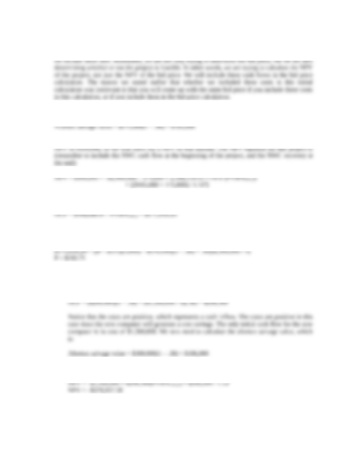
35. We need to find the bid price for a project, but the project has extra cash flows. Since we don’t
already produce the keyboard, the sales of the keyboard outside the contract are relevant cash flows.
Since we know the extra sales number and price, we can calculate the cash flows generated by these
sales. The cash flow generated from the sale of the keyboard outside the contract is:
1 2 3 4
Sales $2,394,000 $2,835,000 $3,759,000 $2,184,000
Variable costs 1,311,000 1,552,500 2,058,500 1,196,000
So, the addition to NPV of these market sales is:
CHAPTER 10 – 8
You may have noticed that we did not include the initial cash outlay, depreciation, or fixed costs in
the calculation of cash flows from the market sales. The reason is that it is irrelevant whether or not
Next, we need to calculate the aftertax salvage value, which is:
Instead of solving for a zero NPV as is usual in setting a bid price, the company president requires an
Solving for the OCF, we get:
Now we can solve for the bid price as follows:
OCF = $171,818.29 = [(P – v)Q – FC ](1 – TC) + TCD
36. a. Since the two computers have unequal lives, the correct method to analyze the decision is the
EAC. We will begin with the EAC of the new computer. Using the depreciation tax shield
approach, the OCF for the new computer system is:
Notice that the costs are positive, which represents a cash inflow. The costs are positive in this
case since the new computer will generate a cost savings. The only initial cash flow for the new
computer is its cost of $1,560,000. We next need to calculate the aftertax salvage value, which
is:
Now we can calculate the NPV of the new computer as:
CHAPTER 10 – 9
And the EAC of the new computer is:
Analyzing the old computer, the only OCF is the depreciation tax shield, so:
The initial cost of the old computer is a little trickier. You might assume that since we already
own the old computer there is no initial cost, but we can sell the old computer, so there is an
This is the initial cost of the old computer system today because we are forgoing the
Now we can calculate the NPV of the old computer as:
And the EAC of the old computer is:
CHAPTER 10 – 10
b. If we are only concerned with whether or not to replace the machine now, and are not worrying
about what will happen in two years, the correct analysis is NPV. To calculate the NPV of the
decision on the computer system now, we need the difference in the total cash flows of the old
computer system and the new computer system. From our previous calculations, we can say the
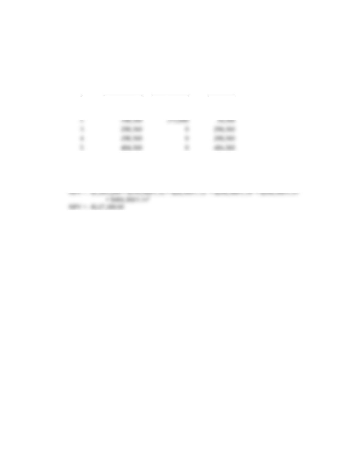
cash flows for each computer system are:
tNew computer Old computer Difference
0 –$1,560,000 –$556,800 –$1,003,200
1 298,360 98,800 199,560
Since we are only concerned with marginal cash flows, the cash flows of the decision to replace
the old computer system with the new computer system are the differential cash flows. The
NPV of the decision to replace, ignoring what will happen in two years is:
If we are not concerned with what will happen in two years, we should not replace the old
computer system.
