LAWN KING, INC.:Sales and Operations Planning
Teaching Notes
1
Synopsis and Purpose
Lawn King is a manufacturer of lawn mowers facing a highly seasonal demand for its products.
At the present time the demand forecast for the coming year has just been increased. This is
Discussion Questions
1. Develop a forecast to use as a basis for S&OP.
2. Develop an S&OP plan by month for fiscal 2015. Consider the use of several different
production strategies. Which strategy do you recommend? Hint: Use of Excel will
The projected increase from FY14 to FY15 is:
Thus a larger increase is being projected than was experienced last year.
LAWN KING, INC.:Sales and Operations Planning
Teaching Notes
2
For purposes of analysis we will accept the new forecast of 110,000 units. Although the
projected demand increase is larger than last year’s actual increase, the forecast still appears
reasonable. It may be, however, that marketing is attempting to drive production through a
higher forecast to avoid stockouts. Therefore, we may wish to evaluate a somewhat lower
forecast, as well as the one given in the case.
To construct an S&OP plan we need to forecast aggregate demand by month. This can be
done by assuming the same monthly pattern as last year. From exhibit 4 in the case, the
percentage of annual sales by month can be calculated. These percentages are then multiplied
by the total forecast (110,000) to arrive at monthly demand forecasts. (See Exhibit 1 of the
teaching note.)
While a turnover of 6.7 might be considered good, the inventory level should ideally be
compared to the demand at the end of the year. Since the demand is seasonal, our goal should
be to have 1 or 2 months of inventory at year-end as a safety stock. More inventory is not
necessary, since all models are still in production and we can respond to changing demand
conditions. One month of inventory would amount to 1216 units (the projected demand for
September). Two months of inventory would be 3698 units, the demand for September and
October. By this criterion, a great deal of excess inventory exists. Therefore, we will assume
an 8/31/11 goal of 3700 units (2 months supply) of inventory for the remainder of this analysis.
Adjusting for the inventory change, we have a production requirement of 97,240 units.
Forecast
110,000
Beginning Inventory
– 16,460
Ending Inventory
+ 3,700
Production Required
97,240
There are many alternative strategies to consider. For the sake of simplicity we shall consider
four strategies.
1. Level production
2. Level production with overtime
3. Chase demand
4. Two shifts
LAWN KING, INC.:Sales and Operations Planning
Teaching Notes
3
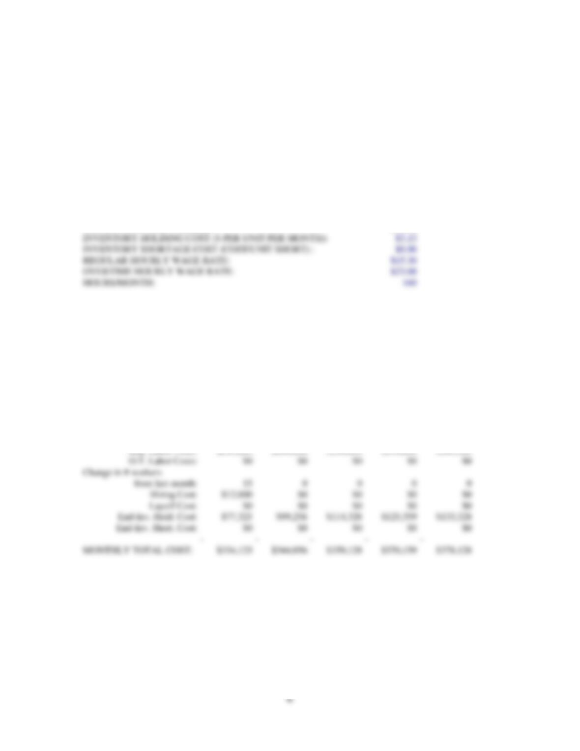
The level production strategy is shown in Exhibit 1 attached. A level of 100 workers is used for
September through February. This level is then phased down to 85 and then to 49 workers at
the end of the year in order to reach an ending inventory of about 3700 units. It is not possible
to use a completely level strategy in this case without significant stockouts or a larger ending
inventory than desired. Thus an arbitrary initial level of 100 workers is selected with a reduction
in work force later in the year. Other levels could also be selected.
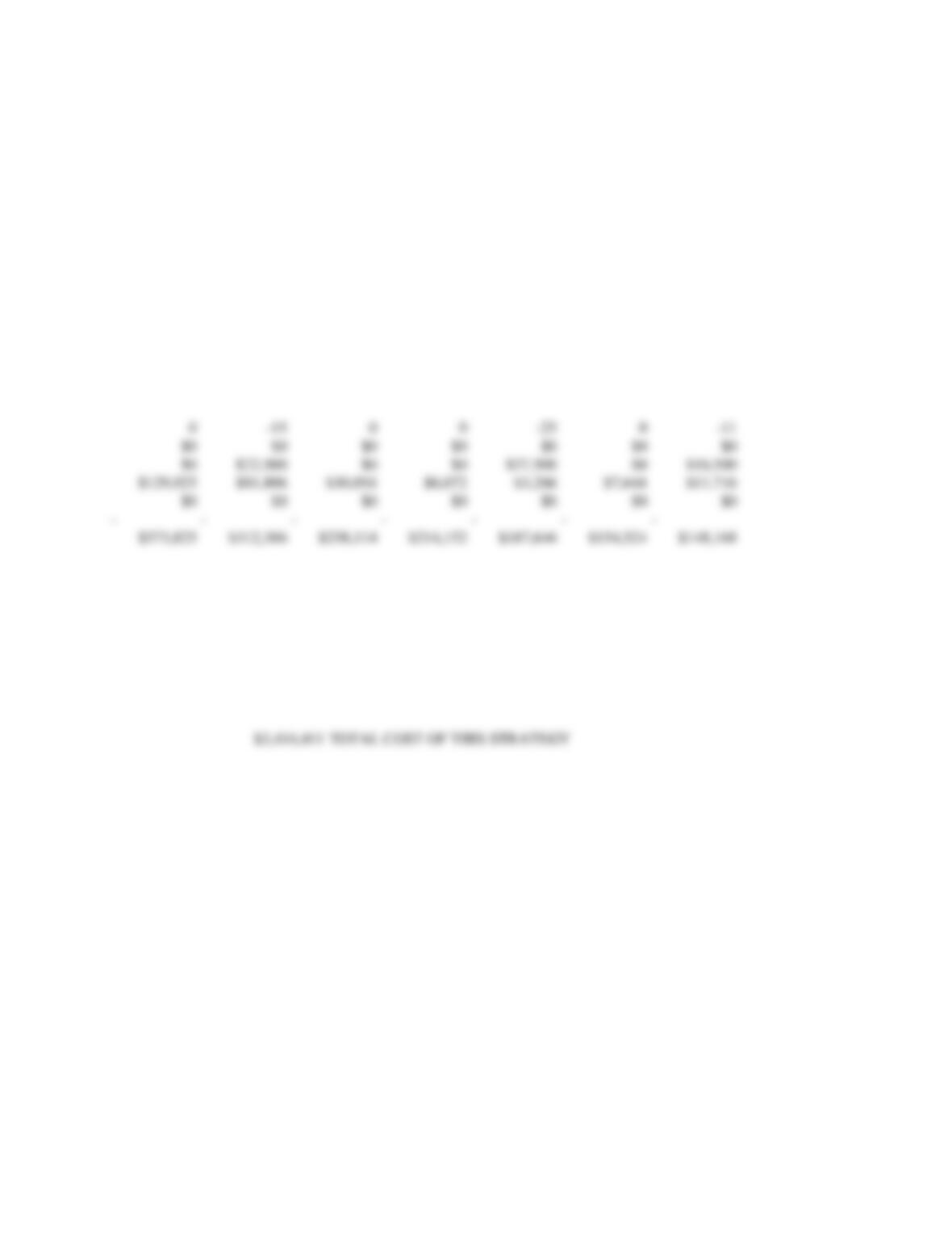
The second strategy, shown in Exhibit 2, is a level strategy with overtime. In this case we
choose a level of 85 regular workers through May, and then phased down to 52 workers at the
end of the year to achieve an ending inventory level of 3700 units. Overtime is used in the
months of December through May to meet the peak demands. Other profiles of level production
and overtime could be selected.
Note, the ending inventory in all strategies should be the same in order to insure a comparable
basis of costing. Students often overlook this point and, as a result, arrive at very different cost
estimates.
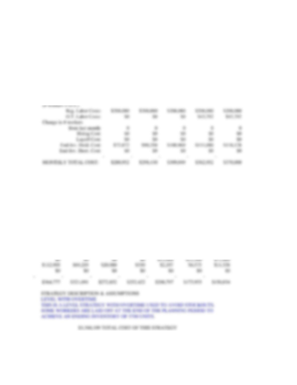
The third strategy is to chase demand as shown in Exhibit 3. The chase strategy matches
demand in Sept through Feb. Then a maximum of 200 workers in used in March and April while
inventory is worked off and the level of workers is phased down to chase demand and end the
year with 3700 units.
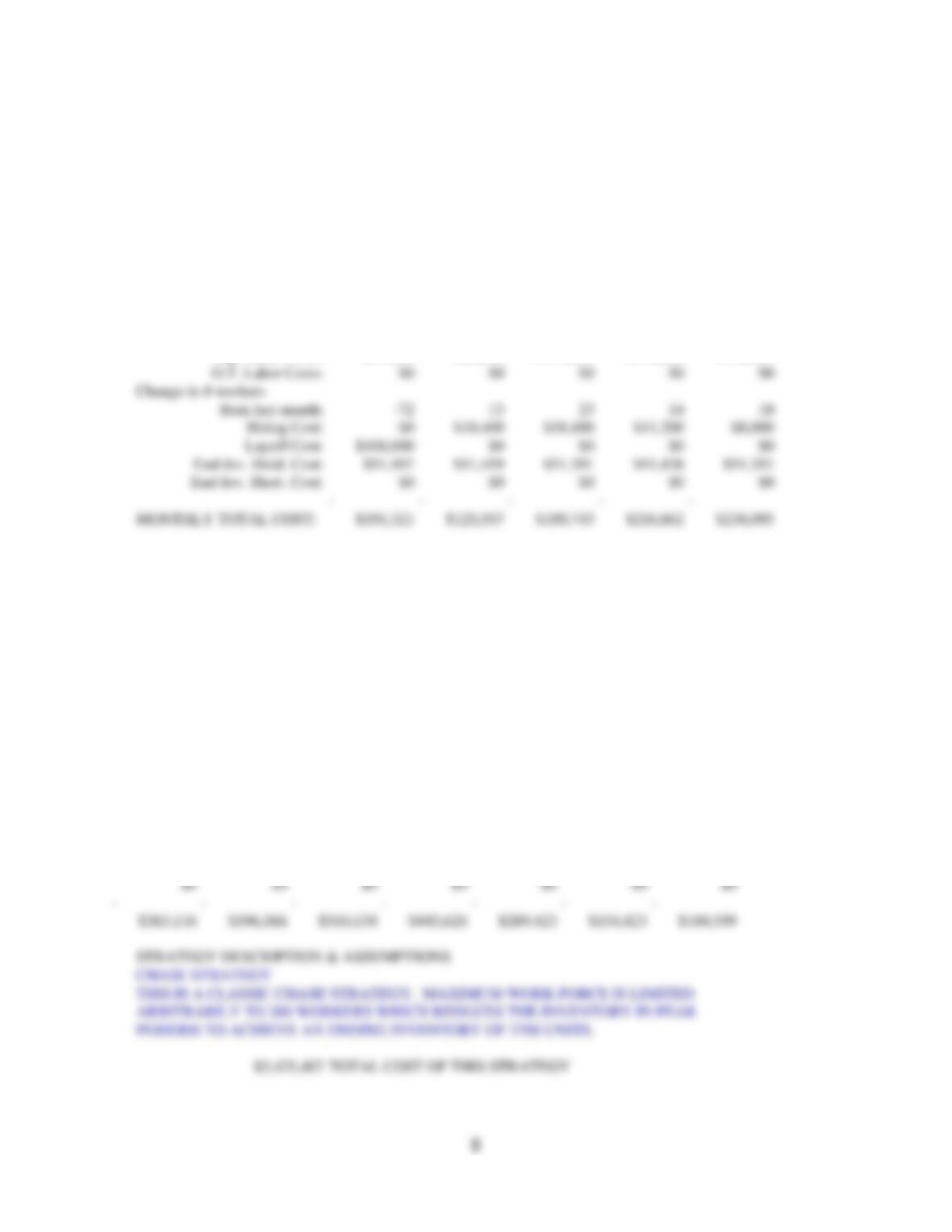
The fourth strategy is a two-shift strategy, shown in Exhibit 4. This strategy starts with a level of
60 workers in Sept through Dec (first shift) and then doubles the level of workers to 120 (second
shift) from Jan through May. The second shift is phased down to arrive at the same ending
inventory as the rest of the strategies.
In order to evaluate these four strategies we will need to make various assumptions about costs
and resources. The first assumption is the nominal production rate of a worker in a month.
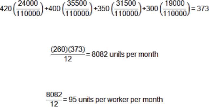
Using the data from Exhibit 4 in the case, an average daily production of 373 units is computed
as the following weighted average:
Since there are 260 production days in a year (52 weeks x 5 days per week), the average
monthly production is 8,082 units:
The initial variable work force level is 85 workers (excludes 10 maintenance and 5 office
workers). The production per direct (or variable) worker is therefore:
LAWN KING, INC.:Sales and Operations Planning
Teaching Notes
The hiring cost per worker is $800 and the layoff cost is $1500 per worker as given in the case.
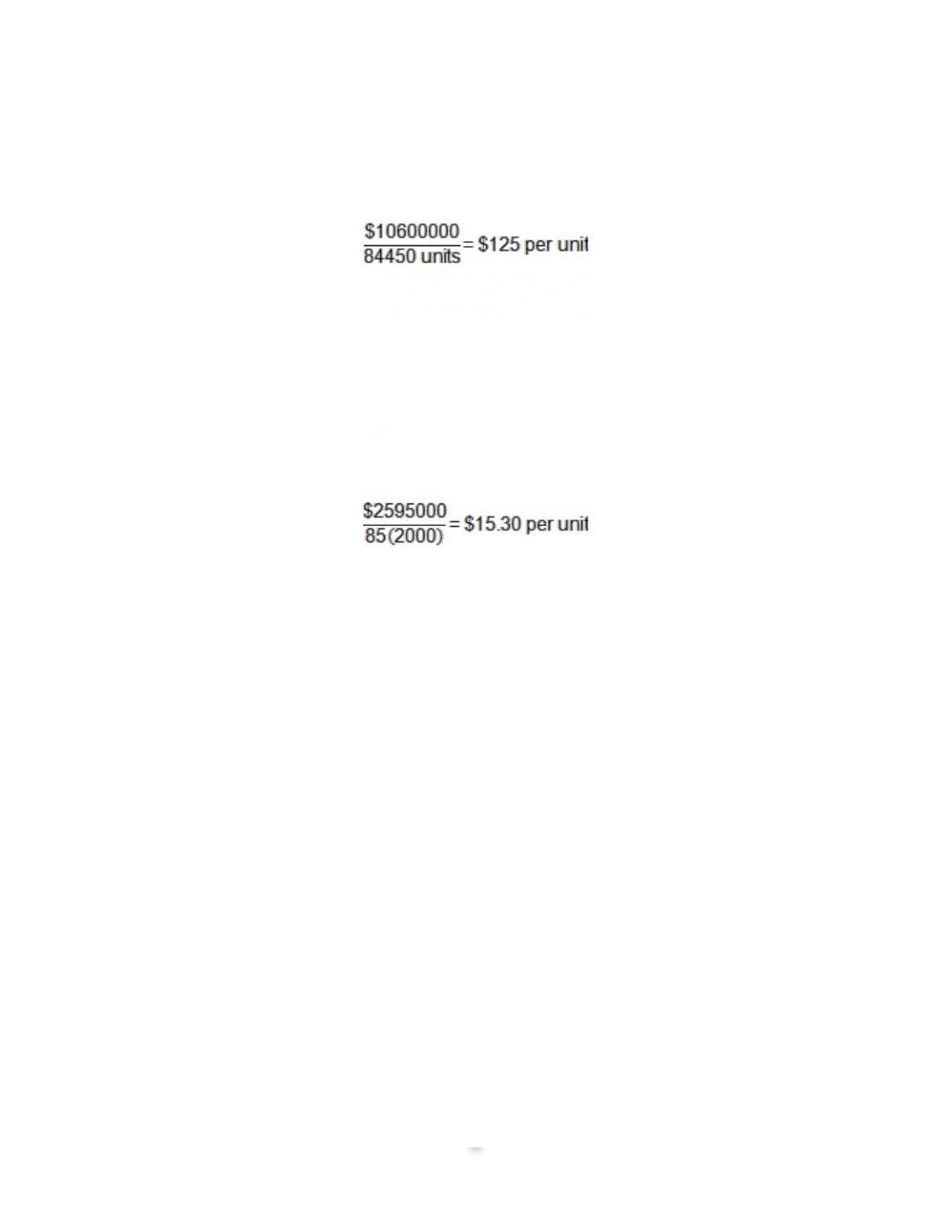
To calculate inventory carrying cost, we need to know the cost of producing a unit. Using labor
and material costs for FY10, we arrive at a unit cost of:
This unit cost is multiplied by 2.5% a month carrying cost (30% a year) to arrive at
$3.125 per unit per month
This unit carrying cost is multiplied by the total inventory carried to arrive at the inventory
carrying cost for each month.
The direct labor cost per hour is obtained by taking the direct labor costs from the Profit and
Loss Statement (Exhibit 1 in the case) and dividing by the number of direct workers (85) times
2000 hours per year as follows:
The overtime rate is 150% of direct labor and thus the overtime rate is 150% times $15.30 =
$23.00 per hour.
In order to calculate the costs of each strategy we use the spreadsheet (file named LAWNKING)
for this case on the website for the textbook. The above cost numbers are input into the
spreadsheet for all of the strategies. Then each strategy is evaluated, one at a time, as shown
in Exhibits 1 to 4.
The result of these cost evaluations is as follows:
Strategy 1: Level
$3,414,411
Strategy 2: Level with Overtime
$3,360,109
Strategy 3: Chase
$3,425,407
Strategy 4: Two-Shift
$3,290,880
As noted above, the two-shift strategy has the lowest cost, by about $70,000 per year, over the
level with overtime strategy. The two-shift strategy is the cheapest, because overtime is more
expensive and it is relatively expensive to hire and lay off workers. In a sense the two-shift
strategy does the best job of fitting the demand profile by using regular workers.
The two-shift strategy not only offers cost advantages, but more flexibility and less inventory risk
than the level strategy. The two-shift strategy is therefore preferred to the level strategy,
provided employees can be found to work a second shift for only part of the year.
While the use of level strategy with overtime is more attractive than a pure level strategy, the
flexibility to meet further demand increases is no longer available once overtime is built into the
S&OP. Especially in view of the fact that a large amount of overtime is needed for strategy 2.

LAWN KING, INC.:Sales and Operations Planning
Teaching Notes
5
The two-shift strategy is also preferred to the chase strategy because it not only costs less but
requires less personnel turmoil. Hiring and layoff is only done once for the two-shift strategy
rather than frequently throughout the year. The chase strategy also implies that the production
line can be easily speeded up and slowed down, while the two shift strategy provides for a
constant line speed.
I think the above arguments provide a compelling case for the two-shift strategy. Lively
arguments can be constructed, however, because the company can “squeak by” without using a
second shift. Also, the two-shift strategy might not be entirely obvious to some students as an
option that should be evaluated.
Teaching Strategy
This case can be taught using the same order of discussion as the above analysis: forecast,
alternative strategies, costing, and recommendation. The case will take one hour or more to
teach depending on how much analysis is put on the board and how much discussion is
encouraged.
This case provides practice in formulating and evaluating S&OP strategies. Management is
facing a dilemma because the sales manager has pushed the forecast a little beyond a one-shift
operation, unless large amounts of overtime or hiring and layoff are used. The demand here is
also very seasonal so flexibility in addition to cost is an important issue in S&OP planning.
There is also the question of how much inventory to carry at the end of the year.
When assigning the case, the students should be warned not to engage in excessive number
crunching. Students can easily become bogged down in developing one schedule after
another, while not reaching a sound conclusion.
LAWN KING, INC.:Sales and Operations Planning
Teaching Notes
EXHIBIT 1 (LEVEL STRATEGY)
FILENAME: LAWNKING
NAME:
KEY
*
SECTION:
*
BASIC INPUT DATA
DATE:
03-Apr
=
MONTHLY PROD. RATE (UNITS/WORKER/MONTH):
95
UNITS
BEGINNING INVENTORY (UNITS):
16460
UNITS
BEGINNING NUMBER OF WORKERS:
85
WORKERS
HIRING COST PER WORKER:
$800
LAYOFF COST PER WORKER:
$1,500
INVENTORY HOLDING COST ($ PER UNIT PER MONTH):
$3.13
INVENTORY SHORTAGE COST (COST/UNIT SHORT) :
$0.00
REGULAR HOURLY WAGE RATE:
$15.30
OVERTIME HOURLY WAGE RATE:
$23.00
HOURS/MONTH:
160
MONTH
SEPT.
OCT.
NOV.
DEC.
JAN.
–
–
–
–
–
Sales Forecast:
1,216
2,482
4,677
5,970
6,950
Units Produced:
9500
9500
9500
9500
9500
Ending Inventory:
24744
31762
36585
40115
42665
Number of Workers:
100
100
100
100
100
Overtime Percent:
0%
0%
0%
0%
0%
Total Equivalent
number of workers:
100
100
100
100
100
(# workers + O.T.)
Reg. Labor Costs:
$244,800
$244,800
$244,800
$244,800
$244,800
O.T. Labor Costs:
$0
$0
$0
$0
$0
Change in # workers
from last month:
15
0
0
0
0
Hiring Cost:
$12,000
$0
$0
$0
$0
Layoff Cost:
$0
$0
$0
$0
$0
End-Inv. Hold. Cost:
$77,325
$99,256
$114,328
$125,359
$133,328
End-Inv. Short. Cost:
$0
$0
$0
$0
$0
–
–
–
–
–
MONTHLY TOTAL COST:
$334,125
$344,056
$359,128
$370,159
$378,128
LAWN KING, INC.:Sales and Operations Planning
Teaching Notes
7
EXHIBIT 1 (continued)
FEB.
MAR.
APR.
MAY
JUNE
JULY
AUG.
–
–
–
–
–
–
–
10,877
23,185
24,642
15,743
6,598
4,299
3,352
9500
8075
8075
8075
5700
5700
4655
41288
26178
9611
1943
1045
2446
3749
100
85
85
85
60
60
49
0%
0%
0%
0%
0%
0%
0%
100
85
85
85
60
60
49
$244,800
$208,080
$208,080
$208,080
$146,880
$146,880
$119,952
$0
$0
$0
$0
$0
$0
$0
0
–15
0
0
–25
0
–11
$0
$0
$0
$0
$0
$0
$0
$0
$22,500
$0
$0
$37,500
$0
$16,500
$129,025
$81,806
$30,034
$6,072
$3,266
$7,644
$11,716
$0
$0
$0
$0
$0
$0
$0
–
–
–
–
–
–
–
$373,825
$312,386
$238,114
$214,152
$187,646
$154,524
$148,168
STRATEGY DESCRIPTION & ASSUMPTIONS
=====================
=========
=========
LEVEL STRATEGY
THIS IS A CLASSICAL LEVEL STRATEGY WITH A REDUCTION IN THE LEVEL
TOWARD THE END OF THE PLANNING PERIOD IN ORDER TO ARRIVE AT AN
ENDING INVENTORY OF 3700 UNITS. THE INITIAL WORK FORCE IS
ARBITRARILY SELECTED TO BE 100 WORKERS.
$3,414,411
TOTAL COST OF THIS STRATEGY
LAWN KING, INC.:Sales and Operations Planning
Teaching Notes
8
EXHIBIT 2 (OVERTIME)
MONTHS:
SEPT.
OCT.
NOV.
DEC.
JAN.
Sales Forecast:
1,216
2,482
4,677
5,970
6,950
Units Produced:
8075
8075
8075
9206
9206
Ending Inventory:
23319
28912
32310
35546
37801
Number of Workers:
85
85
85
85
85
Overtime Percent:
0%
0%
0%
14%
14%
Total Equivalent
number of workers:
85
85
85
96.9
96.9
(# workers + O.T.)
Reg. Labor Costs:
$208,080
$208,080
$208,080
$208,080
$208,080
O.T. Labor Costs:
$0
$0
$0
$43,792
$43,792
Change in # workers
from last month:
0
0
0
0
0
Hiring Cost:
$0
$0
$0
$0
$0
Layoff Cost:
$0
$0
$0
$0
$0
End-Inv. Hold. Cost:
$72,872
$90,350
$100,969
$111,080
$118,128
End-Inv. Short. Cost:
$0
$0
$0
$0
$0
–
–
–
–
–
MONTHLY TOTAL COST:
$280,952
$298,430
$309,049
$362,952
$370,000
FEB.
MAR.
APR.
MAY
JUNE
JULY
AUG.
–
–
–
–
–
–
–
10,877
23,185
24,642
15,743
6,598
4,299
3,352
9206
9206
9206
9206
7125
5700
4940
36130
22150
6714
176
703
2104
3692
85
85
85
85
75
60
52
14%
14%
14%
14%
0%
0%
0%
96.9
96.9
96.9
96.9
75
60
52
$208,080
$208,080
$208,080
$208,080
$183,600
$146,880
$127,296
$43,792
$43,792
$43,792
$43,792
$0
$0
$0
0
0
0
0
–10
–15
–8
$0
$0
$0
$0
$0
$0
$0
$0
$0
$0
$0
$15,000
$22,500
$12,000
$112,905
$69,219
$20,980
$550
$2,197
$6,575
$11,538
$0
$0
$0
$0
$0
$0
$0
–
–
–
–
–
–
–
$364,777
$321,091
$272,852
$252,422
$200,797
$175,955
$150,834
STRATEGY DESCRIPTION & ASSUMPTIONS
LEVEL WITH OVERTIME
THIS IS A LEVEL STRATEGY WITH OVERTIME USED TO AVOID STOCKOUTS.
SOME WORKERS ARE LAID OFF AT THE END OF THE PLANNING PERIOD TO
ACHIEVE AN ENDING INVENTORY OF 3700 UNITS.
$3,360,109
TOTAL COST OF THIS STRATEGY
LAWN KING, INC.:Sales and Operations Planning
Teaching Notes
EXHIBIT 3 (CHASE STRATEGY)
SEPT.
OCT.
NOV.
DEC.
JAN.
Sales Forecast:
1,216
2,482
4,677
5,970
6,950
Units Produced:
1235
2470
4655
5985
6935
Ending Inventory:
16479
16467
16445
16460
16445
Number of Workers:
13
26
49
63
73
Overtime Percent:
0%
0%
0%
0%
0%
Total Equivalent
number of workers:
13
26
49
63
73
(# workers + O.T.)
Reg. Labor Costs:
$31,824
$63,648
$119,952
$154,224
$178,704
O.T. Labor Costs:
$0
$0
$0
$0
$0
Change in # workers
from last month:
–72
13
23
14
10
Hiring Cost:
$0
$10,400
$18,400
$11,200
$8,000
Layoff Cost:
$108,000
$0
$0
$0
$0
End-Inv. Hold. Cost:
$51,497
$51,459
$51,391
$51,438
$51,391
End-Inv. Short. Cost:
$0
$0
$0
$0
$0
–
–
–
–
–
MONTHLY TOTAL COST:
$191,321
$125,507
$189,743
$216,862
$238,095
FEB.
MAR.
APR.
MAY
JUNE
JULY
AUG.
–
–
–
–
–
–
–
10,877
23,185
24,642
15,743
6,598
4,299
3,352
10830
19000
19000
13300
6650
3800
3325
16398
12213
6571
4128
4180
3681
3654
114
200
200
140
70
40
35
0%
0%
0%
0%
0%
0%
0%
114
200
200
140
70
40
35
$279,072
$489,600
$489,600
$342,720
$171,360
$97,920
$85,680
$0
$0
$0
$0
$0
$0
$0
41
86
0
–60
–70
–30
–5
$32,800
$68,800
$0
$0
$0
$0
$0
$0
$0
$0
$90,000
$105,000
$45,000
$7,500
$51,244
$38,166
$20,534
$12,900
$13,063
$11,503
$11,419
$0
$0
$0
$0
$0
$0
$0
–
–
–
–
–
–
–
$363,116
$596,566
$510,134
$445,620
$289,423
$154,423
$104,599
STRATEGY DESCRIPTION & ASSUMPTIONS
CHASE STRATEGY
THIS IS A CLASSIC CHASE STRATEGY. MAXIMUM WORK FORCE IS LIMITED
ARBITRARILY TO 200 WORKERS WHICH REDUCES THE INVENTORY IN PEAK
PERIODS TO ACHIEVE AN ENDING INVENTORY OF 3700 UNITS.
$3,425,407
TOTAL COST OF THIS STRATEGY
Teaching Notes
10
EXHIBIT 4 (TWO-SHIFT STRATEGY)
SEPT.
OCT.
NOV.
DEC.
JAN.
–
–
–
–
–
Sales Forecast:
1,216
2,482
4,677
5,970
6,950
Units Produced:
5700
5700
5700
5700
11400
Ending Inventory:
20944
24162
25185
24915
29365
Number of Workers:
60
60
60
60
120
Overtime Percent:
0%
0%
0%
0%
0%
Total Equivalent
number of workers:
60
60
60
60
120
(# workers + O.T.)
Reg. Labor Costs:
$146,880
$146,880
$146,880
$146,880
$293,760
O.T. Labor Costs:
$0
$0
$0
$0
$0
Change in # workers
from last month:
–25
0
0
0
60
Hiring Cost:
$0
$0
$0
$0
$48,000
Layoff Cost:
$37,500
$0
$0
$0
$0
End-Inv. Hold. Cost:
$65,450
$75,506
$78,703
$77,859
$91,766
End-Inv. Short. Cost:
$0
$0
$0
$0
$0
–
–
–
–
–
MONTHLY TOTAL COST:
$249,830
$222,386
$225,583
$224,739
$433,526
FEB.
MAR.
APR.
MAY
JUNE
JULY
AUG.
–
–
–
–
–
–
–
10,877
23,185
24,642
15,743
6,598
4,299
3,352
11400
11400
11400
11400
8550
4750
4180
29888
18103
4861
518
2470
2921
3749
120
120
120
120
90
50
44
0%
0%
0%
0%
0%
0%
0%
120
120
120
120
90
50
44
$293,760
$293,760
$293,760
$293,760
$220,320
$122,400
$107,712
$0
$0
$0
$0
$0
$0
$0
0
0
0
0
–30
–40
–6
$0
$0
$0
$0
$0
$0
$0
$0
$0
$0
$0
$45,000
$60,000
$9,000
$93,400
$56,572
$15,191
$1,619
$7,719
$9,128
$11,716
$0
$0
$0
$0
$0
$0
$0
–
–
–
–
–
–
–
$387,160
$350,332
$308,951
$295,379
$273,039
$191,528
$128,428
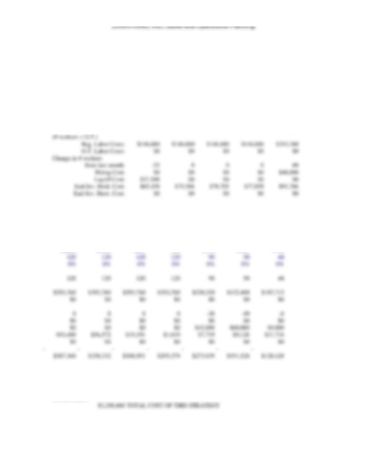
STRATEGY DESCRIPTION & ASSUMPTIONS
A TWO-SHIFT STRATEGY IS USED TO CLOSELY MATCH DEMAND. THE FIRST
SHIFT PROVIDES A TOTAL OF 120 WORKERS. SOME WORKERS ARE LAID-OFF
AT THE END OF THE PLANNING PERIOD TO ARRIVE AT 3700 UNITS IN
INVENTORY.
$3,290,880
TOTAL COST OF THIS STRATEGY