
Chapter 10 – Forecasting
10-1
Chapter 10
Forecasting
Teaching Notes
This chapter presents introductory material on forecasting. The chapter uses qualitative,
time series, and causal forecasting models as a basis for organization. While this chapter is fairly
quantitative, it also presents material on how forecasting methods should be selected and used in
organizations.
When teaching this chapter, we try to illustrate the different uses of forecasting in
operations and the different methods available. We also try to demonstrate the link between uses
and methods before presenting the methods themselves. We stress exponential smoothing in this
chapter, since regression is often covered in other business or statistics courses. It will likely
help students if a few exponential smoothing problems are worked out in class. It may be useful
to present some elementary computerized forecasting systems and some of the problems
associated with using quantitative forecasting methods in practice. Collaborative Planning,
Forecasting, and Replenishment (CPFR) is a popular topic that ties in nicely with supply chain
material and topics.
Answers to Questions
1. Demand is a measure of the amount of goods or services desired by customers. Sales
measures the amount actually purchased by customers. Sales will accurately reflect
2. A forecast is an unbiased estimate of what will happen. Planning is what the planners
3. Qualitative methods may be most appropriate if historical data about past demand are
4. Qualitative forecasts are useful for long-range time horizons and for purposes such as
process design, capacity planning, and facilities location. They are most useful when no
Chapter 10 – Forecasting
10-2
Copyright © 2017 McGraw-Hill Education. All rights reserved. No reproduction or distribution without the prior written consent of
McGraw-Hill Education.
Causal models are useful in the medium term for aggregate planning and budgeting.
They may be useful in the long term if applicable historical data exist and in the short
term if the cost of the method is low relative to its benefits.
5. For inventory and scheduling, there are usually a large number of products to consider
and decisions tend to be repetitive and frequent. Generally the cost required to make a
6. a. Monthly sales of a retail florist: Seasonal, trend, and random.
7. Exponential smoothing requires less storage of data than the moving average methods.
8. The data should be divided into two subsets. The first set should be used to try different
9. Fit refers to how well a proposed model explains the data points used to determine that
10. The solution to this situation is for marketing and operations to plan and discuss the
forecasts together. First, the purpose of the marketing and operations forecasts should be
discussed to see if this leads to the different forecasts. Perhaps, marketing is using their
11. The purpose of CPFR is to achieve more accurate forecasts by customers and suppliers in
Chapter 10 – Forecasting
10-3
Copyright © 2017 McGraw-Hill Education. All rights reserved. No reproduction or distribution without the prior written consent of
McGraw-Hill Education.
and replenishment plan. The supplier benefits by learning of changes in advertising or
special promotions that the customer is planning, adjustments in the customer’s inventory
or possible demand shifts. The customers benefit in having the suppliers make better use
of their capacity to produce products that the customers will need. Suppliers can also
provide market information or perspectives that the customer might have not have.
12. CPFR is useful when there are a relatively small number of suppliers that provide most of
the product purchased by the customer (80-20 rule). If there are too many suppliers, it
Answers to Problems
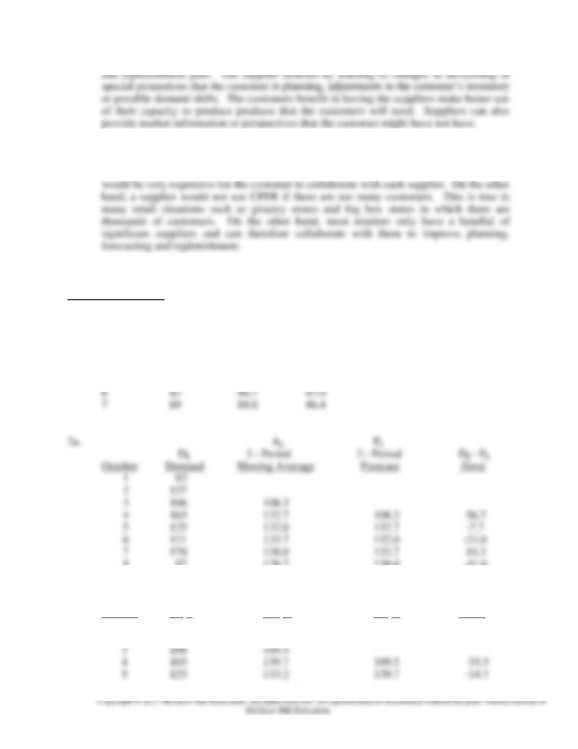
1. Period Demand At(3period) At(5period)
1 85 – –
2 92 – –
3 71 82.7 –
4 97 86.7 –
5 93 87.0 87.6
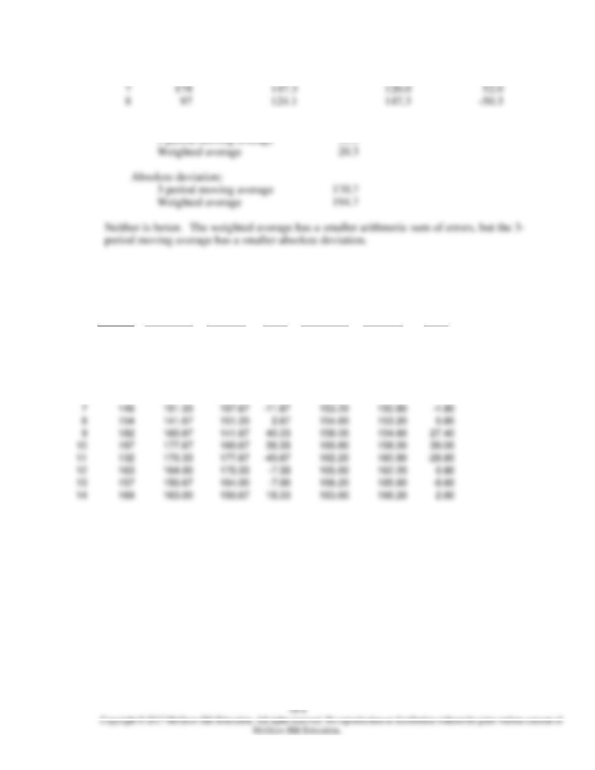
8 97 128.7 138.0 -41.0
2b. Weighted Dt – Ft
October Dt At Ft Error
1 92
2 127
Chapter 10 – Forecasting
6 111 126.0 133.2 -22.2
c. Arithmetic sum of errors:
3 period moving average 31.3
3a.
Day
Dt
Demand
At
3-Period
Mov.Avg.
Ft
3-Period
Forecast
Dt-Ft
Error
At
5-Period
Mov.Avg.
Ft
5-Period
Forecast
Dt-Ft
Error
1
200
2
134
3
147
160.33
4
165
148.67
160.33
4.67
5
183
165.00
148.67
34.33
165.80
6
125
157.67
165.00
–40.00
150.80
165.80
–40.80
7
146
151.33
157.67
–11.67
153.20
150.80
–4.80
8
154
141.67
151.33
2.67
154.60
153.20
0.80
9
182
160.67
141.67
40.33
158.00
154.60
27.40
10
197
177.67
160.67
36.33
160.80
158.00
39.00
11
132
170.33
177.67
–45.67
162.20
160.80
–28.80
12
163
164.00
170.33
–7.33
165.60
162.20
0.80
13
157
150.67
164.00
–7.00
166.20
165.60
–8.60
14
169
163.00
150.67
18.33
163.60
166.20
2.80
10-5
Copyright © 2017 McGraw-Hill Education. All rights reserved. No reproduction or distribution without the prior written consent of
McGraw-Hill Education.
50
100
150
200
250
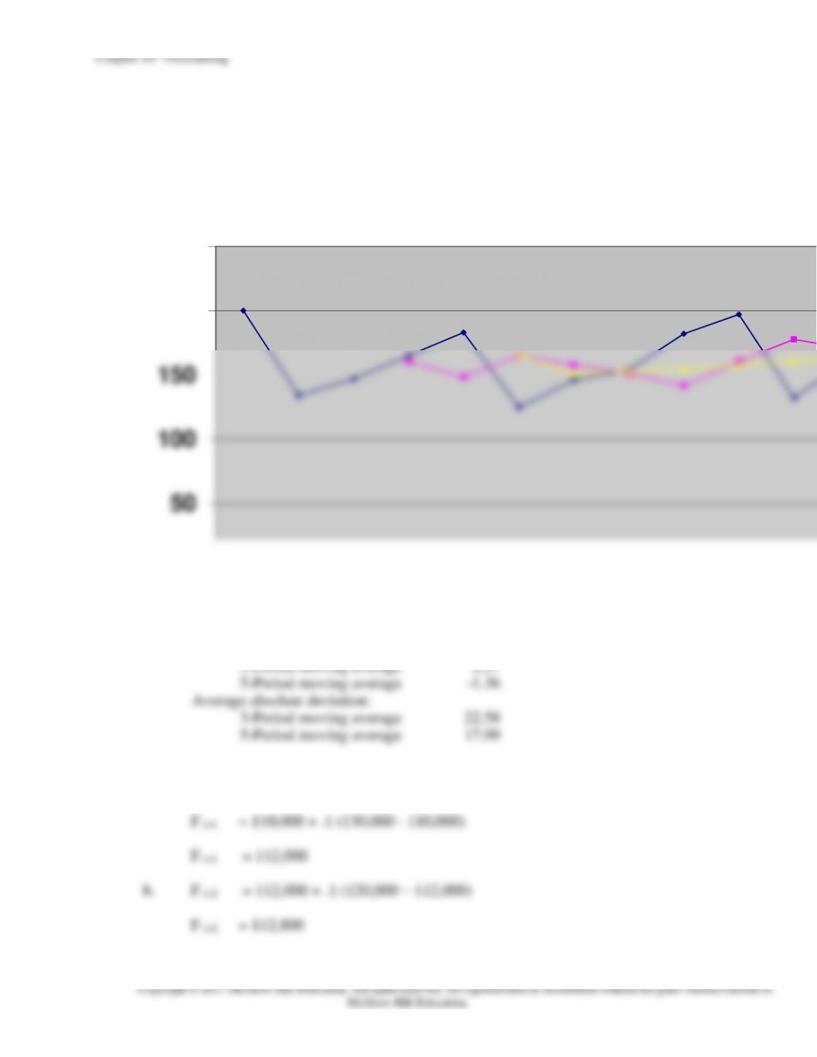
Problem 3b. Demand and Forecasts
c. The 5-period moving average is better because it smoothes the wide demand swings. It
also performs better according to the measures listed below:
Arithmetic mean of errors:
4. a. F t+1 = F t + (D t – F t)
Chapter 10 – Forecasting
10-6
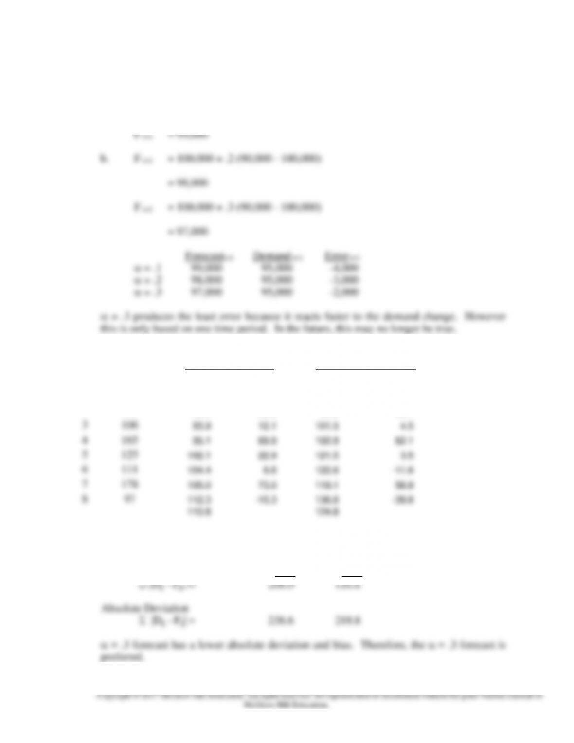
5. a. Ft+1 = F t + (D t – F t)
F t+1 = 100,000 + .1 (90,000 – 100,000)
6. = .1 = .3
Period Dt Ft Dt – Ft Ft Dt – Ft
1
92
90
2
90
2
2
127
90.2
36.8
90.6
36.4
3
106
93.9
12.1
101.5
4.5
4
165
95.1
69.9
102.9
62.1
5
125
102.1
22.9
121.5
3.5
6
111
104.4
6.6
122.6
–11.6
7
178
105.0
73.0
119.1
58.9
8
97
112.3
–15.3
136.8
–39.8
110.8
124.8
7. Refer to problem # 6.
Arithmetic Sum (Bias Error) = .1 = .3

Chapter 10 – Forecasting
10-7
8a.
NAME:
****************
CHAPTER 10 PROBLEM 8
SEC:
**********
ALPHA
0.1
Tracking
Absolute
CumSum
Day
Demand
Forecast
Error
MAD
Signal
Error
Error
1
200
100.0
100.0
10.0
10.0
100.0
100.0
2
134
110.0
24.0
11.4
10.9
24.0
124.0
3
147
112.4
34.6
13.7
11.6
34.6
158.6
4
165
115.9
49.1
17.3
12.0
49.1
207.7
5
183
120.8
62.2
21.8
12.4
62.2
270.0
6
125
127.0
-2.0
19.8
13.5
2.0
268.0
7
146
126.8
19.2
19.7
14.6
19.2
287.2
8
154
128.7
25.3
20.3
15.4
25.3
312.5
9
182
131.2
50.8
23.3
15.6
50.8
363.2
10
197
136.3
60.7
27.1
15.7
60.7
423.9
11
132
142.4
-10.4
25.4
16.3
10.4
413.5
12
163
141.3
21.7
25.0
17.4
21.7
435.1
13
157
143.5
13.5
23.9
18.8
13.5
448.6
14
169
144.9
24.1
23.9
19.8
24.1
472.8
——–
——–
——-
——-
———
———
——–
TOTALS
2254.0
1781.2
472.8
282.5
203.9
497.5
Chapter 10 – Forecasting
10-8
5
183
144.7
38.3
27.5
6.8
38.3
187.2
6
125
156.2
28.6
5.5
31.2
156.0
7
146
146.8
20.3
7.7
0.8
155.2
8
154
146.6
7.4
16.4
9.9
7.4
162.7
9
182
148.8
33.2
21.5
9.1
33.2
195.9
197
158.8
38.2
26.5
8.8
38.2
234.1
132
170.2
30.0
6.5
38.2
195.9
163
158.8
4.2
22.3
9.0
4.2
200.1
157
160.0
16.5
3.0
197.1
169
159.1
9.9
14.5
14.3
9.9
207.0
——–
——-
——
———
———
——–
TOTALS
319.6
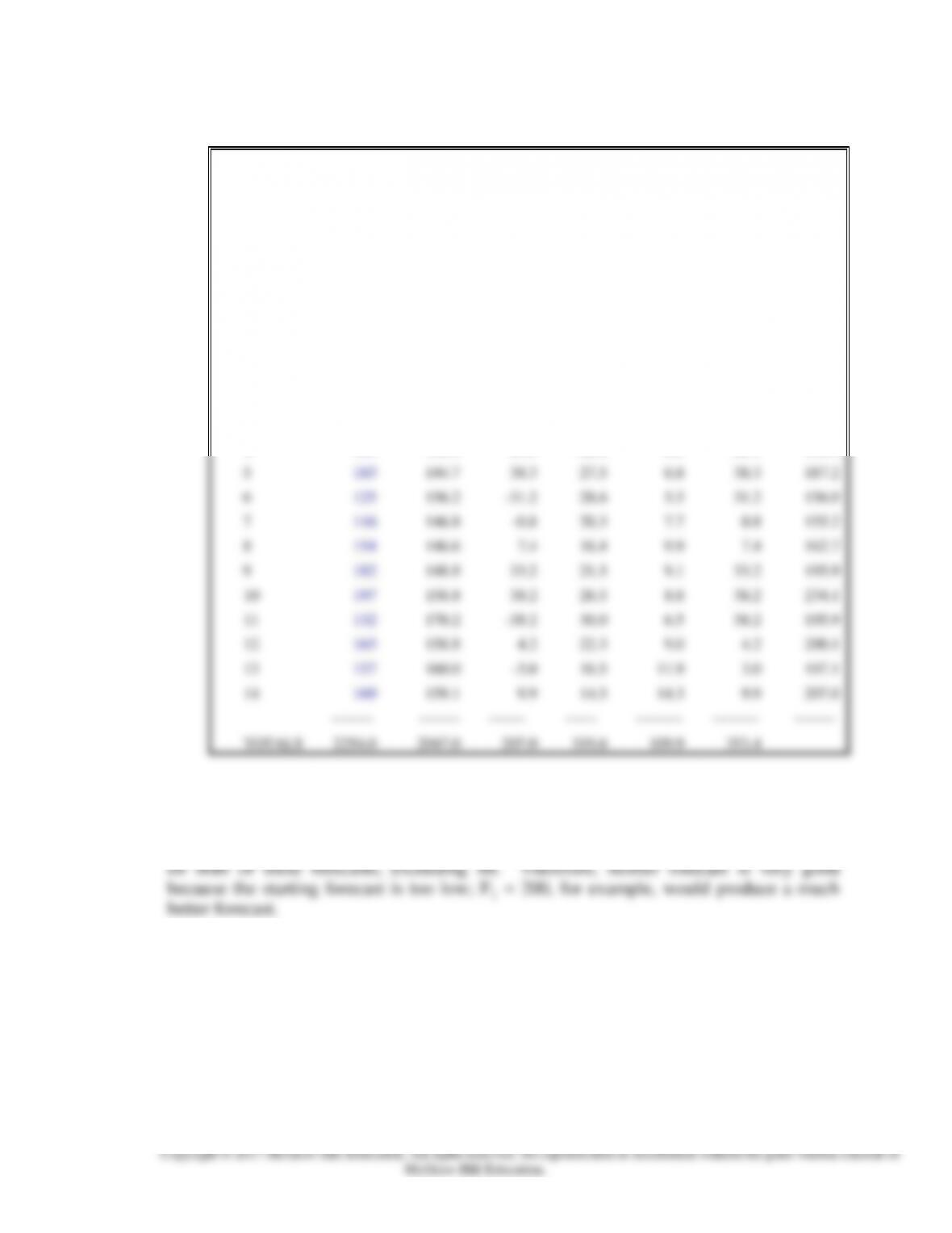
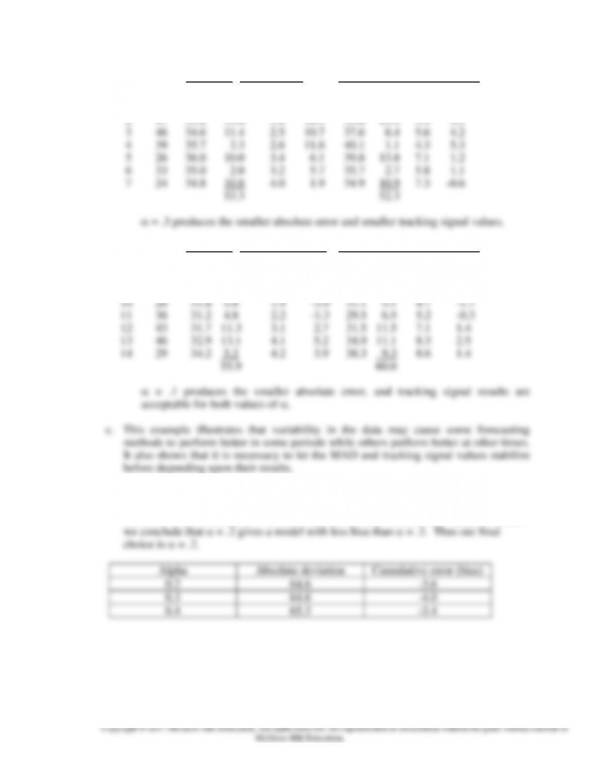
8. a. (continued) Henry’s = .3 produces better results according to the cumulative sum of the
error and cumulative sum of the absolute error. However, the tracking signal is too large
NAME:
****************
CHAPTER 10 PROBLEM 8
SEC:
**********
ALPHA
0.3
Tracking
Absolute
Cum
Sum
Day
Demand
Forecast
Error
MAD
Signal
Error
Error
1
200
100.0
100.0
30.0
3.3
100.0
100.0
2
134
130.0
4.0
22.2
4.7
4.0
104.0
3
147
131.2
15.8
20.3
5.9
15.8
119.8
4
165
135.9
29.1
22.9
6.5
29.1
148.9
Chapter 10 – Forecasting
10-9
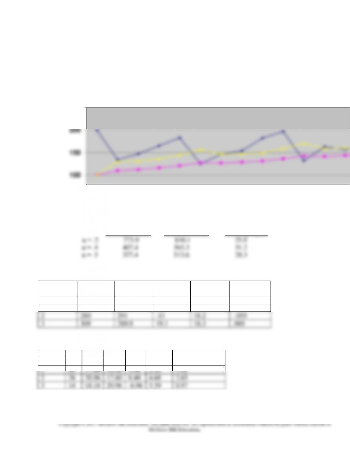
8b.
100
150
200
250
Demand and Forecasts 8b
8. c. Increasing the value of alpha would generally decrease forecast error. However,
without changing the F1 from 100 to a greater value (closer to 200) will simply
bias future forecasts to the low side.
Error Absolute Error Period 14
Cumulative sum Cumulative sum Tracking signal
9.
Period
Dt
Ft
et
MADt
Tracking
Signal
0
20
1
300
290
10
19
.526
2
280
291
-11
18.2
-.055
3
309
289.9
19.1
18.3
.989
10.
Period
Dt
At
Ft
et
MADt
Tracking Signal
0
16.00
1
1
20
17.60
16.00
4.00
2.20
1.82
2
26
20.96
17.60
8.40
4.68
2.65
3
14
18.18
20.96
-6.96
5.59
0.97
Chapter 10 – Forecasting
10-10
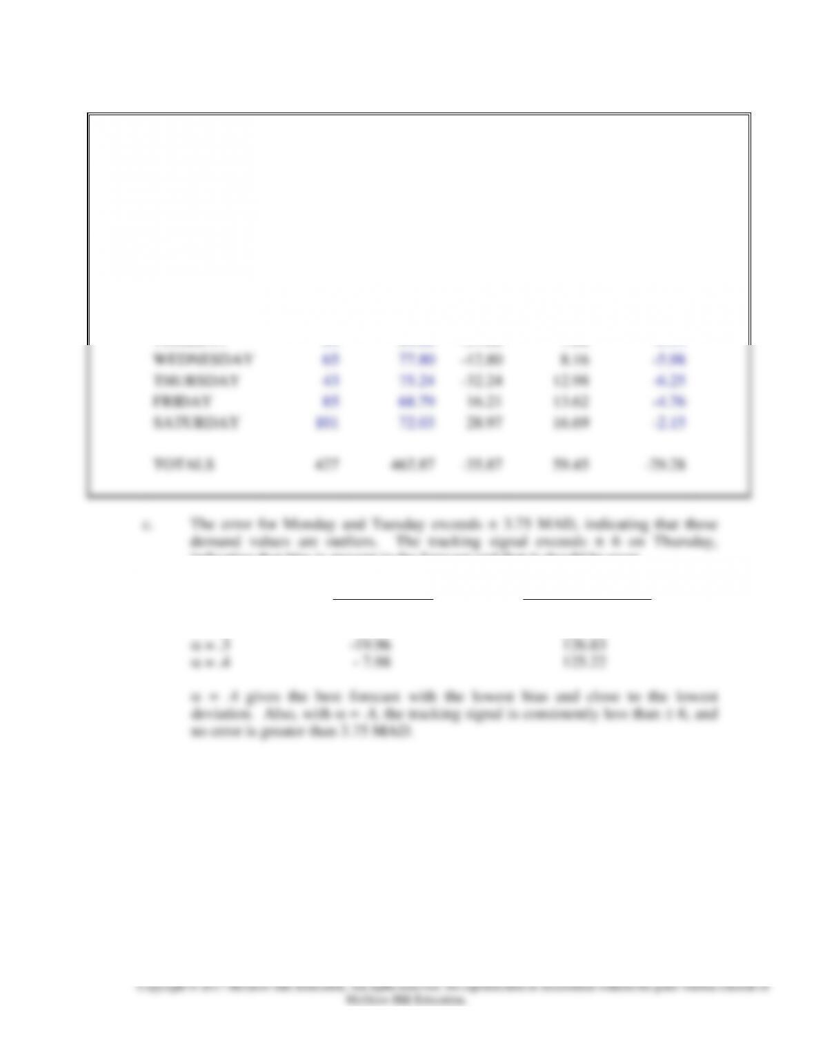
11a and b.
NAME:
**************
CHAPTER 10, PROBLEM 11
SECTION:
**********
ALPHA =
0.2
TRACKING
DEMAND
FORECAST
ERROR
MAD
SIGNAL
MONDAY
80
85.00
-5.00
1.00
-5.00
TUESDAY
53
84.00
-31.00
7.00
-5.14
WEDNESDAY
65
77.80
-12.80
8.16
-5.98
THURSDAY
43
75.24
-32.24
12.98
-6.25
FRIDAY
85
68.79
16.21
13.62
-4.76
SATURDAY
101
72.03
28.97
16.69
-2.15
TOTALS
427
462.87
-35.87
59.45
-29.28
indicating that bias is present in the forecast and that it should be reset.
d. Bias sum errors Sum abs. deviations
= .1 -56.55 122.59
= .2 -35.87 126.22
Chapter 10 – Forecasting
10-11
12a. = .1 = .3
Day Dt Ft et MAD TS Ft et MAD TS
1 35 33.0 2.0 0.2 10.0 33.0 2.0 0.6 3.3
12b. = .1 = .3
Day Dt Ft et MAD TS Ft et MAD TS
8 39 32.0 7.0 0.7 10.0 32.0 7.0 2.1 3.3
9 24 32.7 8.7 1.5 -1.1 34.1 10.1 4.5 -0.7
13. a. From the following output for = .2, = .3, and = .4, the smallest absolute
deviation is at = .2 and = .3, so we look at the bias for these two values of and