
1
CHAPTER 12
DATA ANALYSIS AND INTERPRETATION:
PART II. TESTS OF STATISTICAL SIGNIFICANCE AND THE ANALYSIS STORY
CHAPTER OUTLINE AND OBJECTIVES
I. Overview
II. Null Hypothesis Significance Testing (NHST)
Null hypothesis testing is used to determine whether mean differences among groups in an
experiment are greater than the differences that are expected simply because of error variation.
The first step in null hypothesis testing is to assume that the groups do not differ—that is, that the
independent variable did not have an effect (the null hypothesis).
Probability theory is used to estimate the likelihood of the experiment’s observed outcome, assuming
the null hypothesis is true.
A statistically significant outcome is one that has a small likelihood of occurring if the null hypothesis
were true.
Because decisions about the outcome of an experiment are based on probabilities, errors may occur:
Type I (rejecting a true null hypothesis) or Type II (failing to reject a false null hypothesis).
III. Experimental Sensitivity and Statistical Power
Sensitivity refers to the likelihood that an experiment will detect the effect of an independent variable
when, in fact, the independent variable truly has an effect.
Power refers to the likelihood that a statistical test will allow researchers to reject correctly the null
hypothesis of no group differences.
The power of statistical tests is influenced by the level of statistical significance, the size of the
treatment effect, and the sample size.
The primary way for researchers to increase statistical power is to increase sample size.
Repeated measures designs are likely to be more sensitive and to have more statistical power than
independent groups designs because estimates of error variation are likely to be smaller in repeated
measures designs.
Type ll errors are more common in psychological research using NHST than are Type I errors.
When results are not statistically significant (i.e., p > .05), it is incorrect to conclude that the null
hypothesis is true.
IV. NHST: Comparing Two Means

2
The appropriate inferential test when comparing two means obtained from different groups of subjects
is a t-test for independent groups.
A measure of effect size should always be reported when NHST is used.
The appropriate inferential test when comparing two means obtained from the same subjects (or
matched groups) is a repeated measures (within-subjects) t-test.
A. Independent Groups
B. Repeated Measures Designs
V. Statistical Significance and Scientific or Practical Significance
We must recognize the fact that statistical significance is not the same as scientific significance.
We also must acknowledge that statistical significance is not the same as practical or clinical
significance.
VI. Recommendations for Comparing Two Means
VII. Reporting Results When Comparing Two Means
VIII. Data Analysis Involving More Than Two Conditions
IX. ANOVA for Single-Factor Independent Groups Design
Analysis of variance (ANOVA) is an inferential statistics test used to determine whether an
independent variable has had a statistically significant effect on a dependent variable.
The logic of analysis of variance is based on identifying sources of error variation and systematic
variation in the data.
The F-test is a statistic that represents the ratio of between-group variation to within-group variation in
the data.
The results of the initial overall analysis of an omnibus F-test are presented in an analysis of variance
summary table.
Although analysis of variance can be used to decide whether an independent variable has had a
statistically significant effect, researchers examine the descriptive statistics to interpret the meaning of
the experiment’s outcome.
Effect size measures for independent groups designs include eta squared (η2) and Cohen’s f.
A power analysis for independent groups designs should be conducted prior to implementing the
study in order to determine the probability of finding a statistically significant effect, and power should
be reported whenever nonsignificant results based on NHST are found.
Comparisons of two means may be carried out to identify specific sources of systematic variation

3
contributing to a statistically significant omnibus F-test.
A. Calculating Effect Size for Designs with Three or More Independent Groups
B. Assessing Power for Independent Groups Designs
C. Comparing Means in Multiple-Group Experiments
X. Repeated Measures Analysis of Variance
The general procedures and logic for null hypothesis testing using repeated measures analysis of
variance are similar to those used for independent groups analysis of variance.
Before beginning the analysis of variance for a complete repeated measures design, a summary
score (e.g., mean, median) for each participant must be computed for each condition.
Descriptive data are calculated to summarize performance for each condition of the independent
variable across all participants.
The primary way that analysis of variance differs for repeated measures is in the estimation of error
variation, or residual variation; residual variation is the variation that remains when systematic
variation due to the independent variable and subjects is removed from the estimate of total variation.
XI. Two-Factor Analysis of Variance for Independent Groups Designs
A. Analysis of a Complex Design with an Interaction Effect
If the omnibus analysis of variance reveals a statistically significant interaction effect, the source
of the interaction effect is identified using simple main effects analyses and comparisons of two
means.
A simple main effect is the effect of one independent variable at one level of a second
independent variable.
If an independent variable has three or more levels, comparisons of two means can be used to
examine the source of a simple main effect by comparing means two at a time.
Confidence intervals may be drawn around group means to provide information regarding the
precision of estimation of population means.
B. Analysis with No Interaction Effect
If an omnibus analysis of variance indicates the interaction effect between independent variables
is not statistically significant, the next step is to determine whether the main effects of the
variables are statistically significant.
The source of a statistically significant main effect can be specified more precisely by performing
comparisons that compare means two at a time and by constructing confidence intervals.
4
C. Effect Sizes for Two-Factor Design with Independent Groups
XII. Role of Confidence Intervals in the Analysis of Complex Designs
XIII. Two-Factor Analysis of Variance for a Mixed Design
XIV. Reporting Results of a Complex Design
XV. Summary
REVIEW QUESTIONS AND ANSWERS
These review questions appear in the textbook (without answers) at the end of Chapter 12, and can be
used for a homework assignment or exam preparation. Answers to these questions appear in italic.
1. What does it mean to say that results of a statistical test are “statistically significant”?
2. Differentiate between Type l and Type ll errors as they occur when carrying out NHST.
3. What three factors determine the power of a statistical test? Which factor is the primary one that
researchers can use to control power?
4. Why is a repeated measures design likely to be more sensitive than a random groups design?
5. Describe an advantage of using measures of effect size, and explain how power analysis may be
used when a finding is not statistically significant.
6
CHALLENGE QUESTIONS AND ANSWERS
These questions appear in the textbook at the end of Chapter 12, and can be used for a homework
assignment, in-class-discussion, or exam preparation. Answers to these questions appear in italic below.
[Answer to Challenge Question 1 also appears in the text.]
1. A researcher conducts an experiment comparing two methods of teaching young children to read. An
older method is compared with a newer one, and the mean performance of the new method was
found to be greater than that of the older method. The results are reported as t(120) = 2.10, p = .04 (d
= .34).
A. Is the result statistically significant?
B. How many participants were in this study?
C. Based on the effect size measure, d, what may we say about the size of the effect found in this
study?
D. The researcher states that on the basis of this result the newer method is clearly of practical
significance when teaching children to read and should be implemented right away. How would
you respond to this statement?
E. What would the construction of confidence intervals add to our understanding of these results?
2. A social psychologist compares three kinds of propaganda messages on college students’ attitudes
toward the war on terrorism. Ninety (N = 90) students are randomly assigned in equal numbers to the
7
three different communication conditions. A paper–and-pencil attitude measure is used to assess
students’ attitudes toward the war after they are exposed to the propaganda statements. An ANOVA
is carried out to determine the effect of the three messages on student attitudes. Here is the ANOVA
Summary Table:
Source Sum of Squares df Mean Square F p
Communication 180.10 2 90.05 17.87 0.000
Error 438.50 87 5.04
A. Is the result statistically significant? Why or why not?
B. What effect size measure can be easily calculated from these results? What is the value of that
measure?
.29.
C. How could doing comparisons of two means contribute to the interpretation of these results?
D. Although the group means are not provided, it is possible from these data to calculate the width of
the confidence interval for the means based on the pooled variance estimate. What is the width of
the confidence interval for the means in this study?
3. A developmental psychologist gives 4th–, 6th-, and 8th-grade children two types of critical thinking tests.
There are 28 children tested at each grade level; 14 received one form (A or B) of the test. The
dependent measure is the percentage correct on the tests. The mean percentage correct for the
children at each grade level and for the two tests is as follows:
Test 4th 6th 8th
Form A 38.14 63.64 80.21
Form B 52.29 68.64 80.93
Here is the ANOVA Summary Table for this experiment:
8
Source Sum of Squares df Mean Square F p
Grade 17698.95 2 8849.48 96.72 .000
Test 920.05 1 920.05 10.06 .002
Grade × Test 658.67 2 329.33 3.60 .032
Error 7136.29 78 91.49
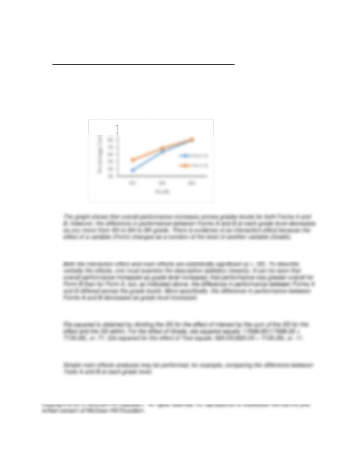
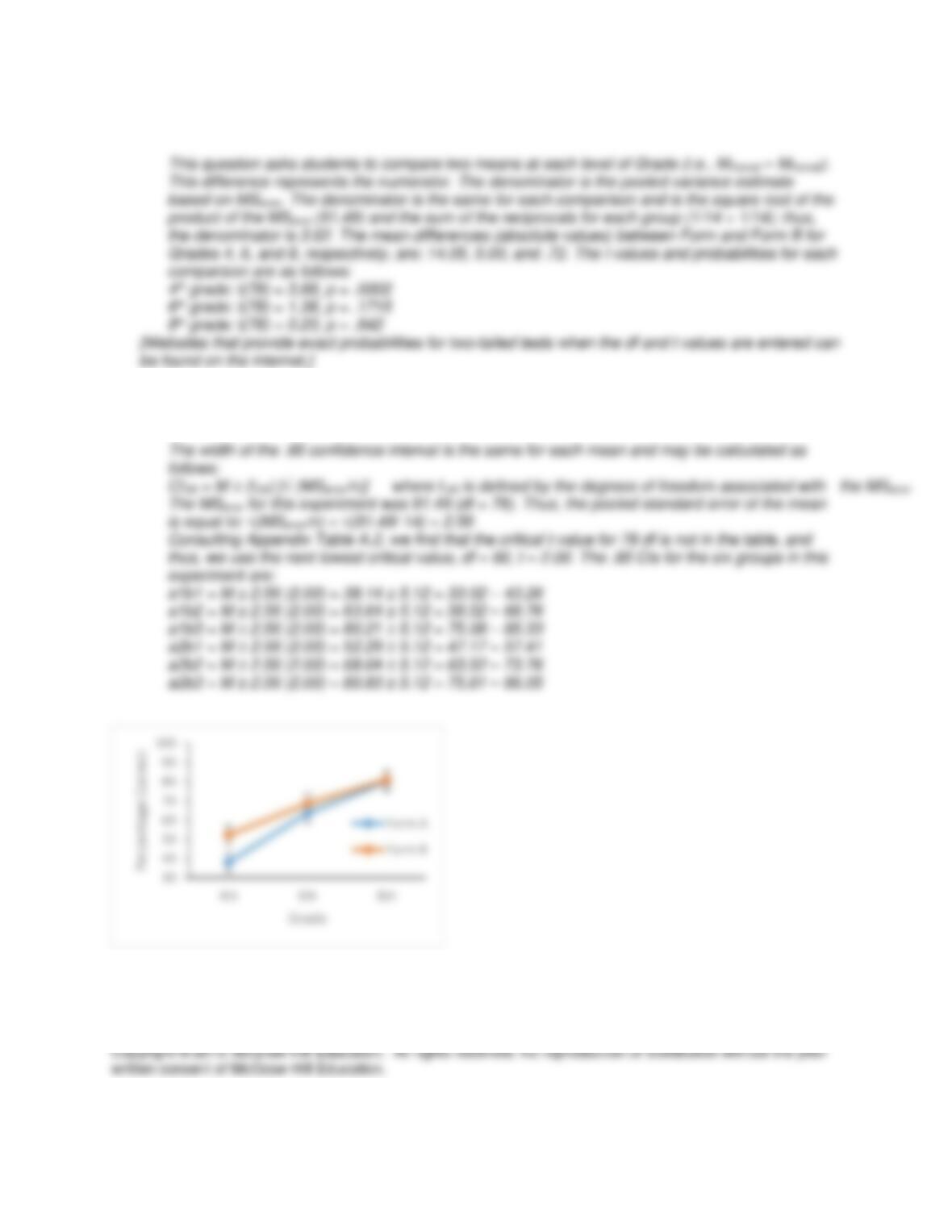
A. Draw a graph showing the mean results for this experiment. Based on your examination of the
graph, would you suspect a statistically significant interaction between the variables? Explain why
or why not.
B. Which effects were statistically significant? Describe verbally each of the significant effects.
C. What are the eta-squared values for the main effects of grade and test?
D. What further analyses could you do to determine the source of the interaction effect?
E. What is the simple main effect of Test for each level of Grade?
90
100
9
10
about Chapter 12 concepts. Material and many exercises from Chapters 6, 7, and 8 are relevant as well.
I. NHST: Comparing Two Means
As we suggested when discussing confidence intervals in Chapter 11, a good place to begin a
discussion of students’ understanding of these concept is to review the True-False test found in the
chapter’s Stretching Exercise. (The answers, without explanation, appear at the end of the chapter).
We present that test below along with an elaboration of the ideas examined. We then present a
different test with True-False questions and answers. Both True-False tests (without answers) are
then presented on separate pages for use in the classroom.
A. Assume that an independent groups design was used to assess performance of participants in an
experimental and control group. There were 12 participants in each condition, and results of
NHST with alpha set at .05 revealed: t(22) = 4.52, p = .006.
True or False? The researcher may reasonably conclude on the basis of this outcome that:
(1) The null hypothesis should be rejected.
(2) The research hypothesis has been shown to be true.
(3) The results are of scientific importance.
(4) The probability that the null hypothesis is true is only .006.
(5) The probability of finding statistical significance at the .05 level if the study were replicated is
greater than if the exact probability had been .02.
B. Following this discussion an instructor may wish to test students’ understanding of NHST when p
> .05 (in this example, p = .06). The above problem can be restated as
Assume that an independent groups design was used to assess performance of participants in an
experimental and control group. There were 12 participants in each condition and results of
NHST with alpha set at .05 revealed: t(22) = 2.02, p = .06.
True or False? The researcher may reasonably conclude on the basis of this outcome that:
(1) The null hypothesis should be rejected.
(2) The null hypothesis has been shown to be true.
(3) The results are of not of scientific importance.
12

13
NHST: Comparing Two Means
A. Decide whether the following statements are true or false for the results of this hypothetical research
and explain your answer.
Assume that an independent groups design was used to assess performance of participants in an
experimental and control group. There were 12 participants in each condition and results of NHST
with alpha set at .05 revealed: t(22) = 4.52, p = .006.
True or False? The researcher may reasonably conclude on the basis of this outcome that:
(1) The null hypothesis should be rejected.
(2) The research hypothesis has been shown to be true.
(3) The results are of scientific importance.
(4) The probability that the null hypothesis is true is only .006.
(5) The probability of finding statistical significance at the .05 level if the study were replicated is
greater than if the exact probability had been .02.
B. Decide whether the following statements are true or false for the results of this hypothetical research
(the probability associated with the t statistic is changed) and explain your answer.
Assume that an independent groups design was used to assess performance of participants in an
experimental and control group. There were 12 participants in each condition and results of NHST
with alpha set at .05 revealed: t(22) = 2.02, p = .06.
True or false? The researcher may reasonably conclude on the basis of this outcome that:
(1) The null hypothesis should be rejected.
(2) The null hypothesis has been shown to be true.
(3) The results are of not of scientific importance.
(4) The probability that the null hypothesis is false is .94 (i.e., 1.00 – .06).
(5) The probability of finding statistical significance at the .05 level if the study were replicated is
much less than if the results had been p = 04.
14
II. Learning to “Read” ANOVA Summary Tables
Today’s students are likely to use a statistical software program to carry out an analysis of variance
(ANOVA). Of course, it is important that students be able to interpret correctly computer output for an
ANOVA and they need practice doing this. In what follows we provide two examples of ANOVA
summary tables with questions based on the information in the tables. These tables are also
reproduced on subsequent pages should instructors wish to do this exercise in a classroom. Similar
problems may be found in the students’ Online Learning Center.
A. Results of a single-factor independent groups design are as follows:
Source Sum of Squares df Mean Square F p
Factor A 440.00 4 110.00 3.65 0.01
Error 1808.40 60 30.14
1. How many levels of Factor A were there?
2. What was the total number of subjects in the experiment?
3. Assuming an equal number of subjects in each group, what was the group size?
4. Were the results of the omnibus F–test statistically significant?
5. (a) What does the researcher know on the basis of this result? and (b) What does the
researcher not know based on this result?
B. Results of a complex independent groups design are as follows:
Source Sum of Squares df Mean Square F p
15
Factor A 159.39 2 79.69 17.52 .000
Factor B 8.03 1 8.03 1.76 .194
A X B 53.72 2 26.86 5.90 .007
Error 136.50 30 4.55
1. How many levels of Factor A are there?
2. How many levels of Factor B are there?
3. What is the total number of subjects?
4. Assuming equal group size, how many subjects are there in each group?
5. What values are used for the numerator and denominator of the F-ratio for each effect?
6. Which results are statistically significant?
7. What analyses are required to specify more clearly the sources of variation contributing to the
interaction effect?

16
Learning to “Read” an ANOVA Summary Table
A. Results of a single-factor independent groups design are as follows:
Source Sum of Squares df Mean Square F p
Factor A 440.00 4 110.00 3.65 0.01
Error 1808.40 60 30.14
1. How many levels of Factor A were there?
2. What was the total number of subjects in the experiment?
3. Assuming an equal number of subjects in each group, what was the group size?
4. Were the results of the omnibus F–test statistically significant?
5. (a) What does the researcher know on the basis of this result?
(b) What does the researcher not know based on this result?
B. Results of a complex independent groups design are as follows:
Source Sum of Squares df Mean Square F p
Factor A 159.39 2 79.69 17.52 .000
Factor B 8.03 1 8.03 1.76 .194
A X B 53.72 2 26.86 5.90 .007
Error 136.50 30 4.55
1. How many levels of Factor A are there?
2. How many levels of Factor B are there?
3. What is the total number of subjects?
4. Assuming equal group size, how many subjects are there in each group?
5. What values are used for the numerator and denominator of the F-ratio for each effect?
6. Which results are statistically significant?
7. What analyses are required to specify more clearly the sources of variation contributing to the
interaction?

17
INSTRUCTOR’S LECTURE/DISCUSSION AIDS
The following pages reproduce content from Chapter 12 and may be used to facilitate lecture or
discussion.
1. Confirmatory Data Analysis: This page focuses on Stage 3 of data analysis, particularly Null
Hypothesis Significance Testing (NHST).
2. Interpreting NHST: This page outlines what researchers learn when making decisions based on
NHST, and defines Type I and Type II errors.
3. Experimental Sensitivity and Statistical Power: Sensitivity and power are defined on this page.
4. NHST: Comparing Two Means: The steps for testing the difference between two independent means
are outlined on this page.
5. Significance: Statistical significance is contrasted with scientific significance and practical/clinical
significance on this page.
6. Recommendations for Comparisons of Two Means: This page summarizes the steps for the statistical
analysis of two means.
7. Data Analysis: More than Two Conditions: This page introduces the steps for data analysis in
experiments involving more than two means and focuses on Analysis of Variance.
8. ANOVA: The F-test: The logic of the F-test is described on this page.
9. NHST with ANOVA: This page outlines the steps for NHST using ANOVA and includes an ANOVA
Summary Table for a single-factor experiment.
10. Effect Size and ANOVA: The procedures for obtaining a measure of effect size following an ANOVA
are described on this page.
11. Describing Effects in Multi-Group Experiments: This page identifies procedures for comparing means
two at a time following a statistically significant omnibus F-test.
12. Repeated Measures ANOVA: This page briefly describes ANOVA for repeated measures, including
the concept of residual variation.
13. ANOVA for Complex Designs: Steps for ANOVA with complex designs are described on this page.
14. Reporting Results of a Complex Design: This page lists key information to include when reporting
results of a complex design.