
1
CHAPTER 11
DATA ANALYSIS AND INTERPRETATION:
PART I. DESCRIBING DATA, CONFIDENCE INTERVALS, CORRELATION
CHAPTER OUTLINE AND OBJECTIVES
I. Overview
II. The Analysis Story
When data analysis is completed, we must construct a coherent narrative that explains our findings,
counters opposing interpretations, and justifies our conclusions.
III. Computer-Assisted Data Analysis
Researchers typically use computers to carry out the statistical analysis of data.
In order to carry out statistical analyses using computer software, researchers must have good
knowledge of research design and statistics.
IV. Illustration: Data Analysis for an Experiment Comparing Means
A. Stage 1: Getting to Know the Data
We begin data analysis by examining the general features of the data and edit or “clean” the data
as necessary.
It is important to check carefully for errors such as missing or impossible values (e.g., numbers
outside the range of a given scale), as well as outliers.
A stem-and-leaf display is particularly useful for visualizing the general features of a data set and
for detecting outliers.
Data can be effectively summarized numerically, pictorially, or verbally; good descriptions of data
frequently use all three modes.
B. Stage 2: Summarizing the Data
Measures of central tendency include the mean, median, and mode.
Important measures of dispersion or variability are the range and standard deviation.
The standard error of the mean is the standard deviation of the theoretical sampling distribution of
means and is a measure of how well we have estimated the population mean.
Effect size measures are important because they provide information about the strength of the
relationship between the independent variable and the dependent variable that is independent of
sample size.

2
An important effect size measure when comparing two means is Cohen’s d.
C. Stage 3: Using Confidence Intervals to Confirm What the Data Reveal
An important approach to confirming what the data are telling us is to construct confidence
intervals for the population parameter, such as a mean or difference between two means.
V. Illustration: Data Analysis for a Correlational Study
A correlation exists when two different measures of the same people, events, or things vary
together—that is, when scores on one variable covary with scores on another variable.
A. Stage 1: Getting to Know the Data
B. Stage 2: Summarizing the Data
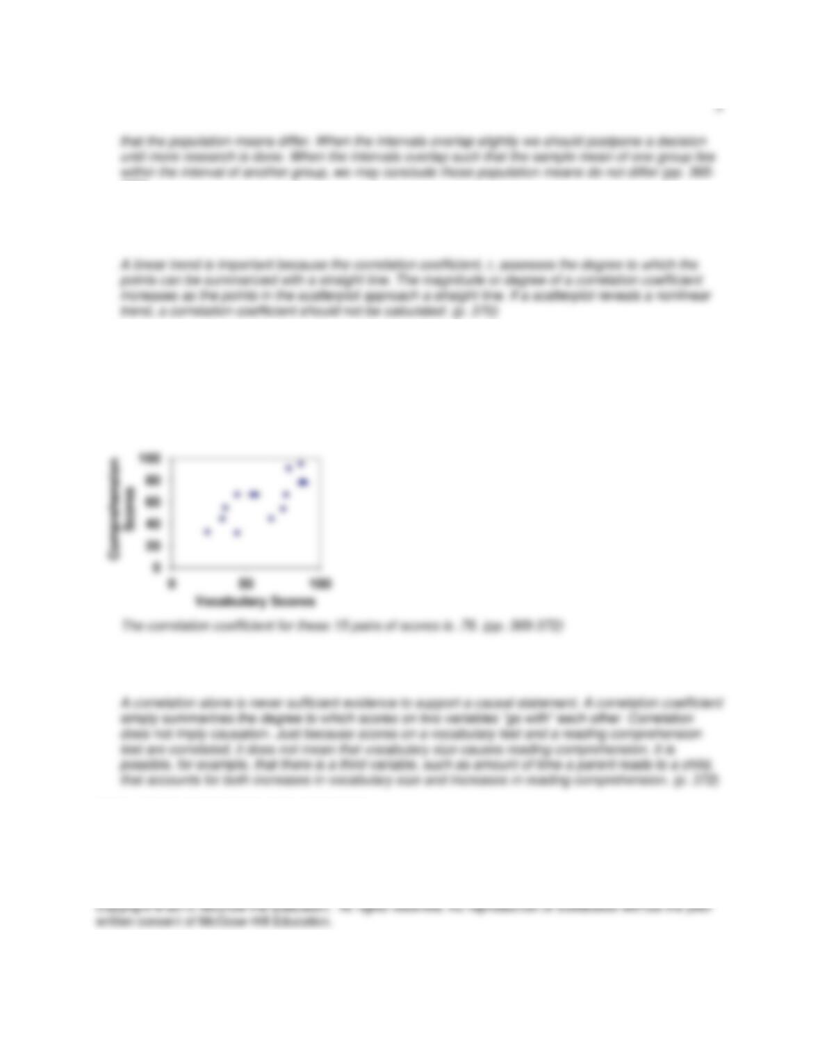
The major descriptive techniques for correlational data are the construction of a scatterplot and
the calculation of a correlation coefficient.
The magnitude or degree of correlation is seen in a scatterplot by determining how well the points
correspond to a straight line; stronger correlations more clearly resemble a straight line (linear
trend) of points.
The magnitude of a correlation coefficient ranges from -1.0 (a perfect negative relationship) to
+1.0 (a perfect positive relationship); a correlation coefficient of 0.0 indicates no relationship.
C. Stage 3: Constructing a Confidence Interval for a Correlation
We can obtain a confidence interval estimate of the population correlation, ρ, just as we did for
the population mean, μ.
VI. Summary
REVIEW QUESTIONS AND ANSWERS
These review questions appear in the textbook (without answers) at the end of Chapter 11, and can be
used for a homework assignment or exam preparation. Answers to these questions appear in italic.
1. Identify the three major stages of data analysis and indicate what specific things a researcher
typically will look to do at each stage.
The three major stages of data analysis are: I. Getting to Know the Data, II. Summarizing the Data,
and III. Confirming What the Data Reveal. In the first stage the researcher inspects the data for errors
and becomes familiar with the general features of the data (e.g., by drawing a figure). In the second
stage the researcher uses descriptive statistics and graphical displays to summarize the data. What
trends and patterns in the data are there? In the third stage, the researcher seeks to confirm what the
data tell us about behavior. Do the results differ from what might be expected by chance? What can
we claim based on the evidence? (p. 344)
2. What does a researcher attempt to do when constructing an “analysis story” to go with the results of a
study?
3. Why must a researcher have a good knowledge of research methodology and statistical procedures
to be able to use computer software to analyze results of a study?
346)
4. Construct a stem-and-leaf display for the following set of numbers; then, report what you have
learned by examining the data in this way. 36, 42, 25, 26, 26, 21, 22, 43, 40, 69, 21, 21, 23, 31, 32,
32, 34, 37, 37, 38, 43, 20, 21, 24, 23, 42, 24, 21, 27, 29, 34, 30, 41, 25, 28
5. Calculate the mean, median, and mode for the following data set: 7,7,2,4,2,4,5,6,4,5. Describe the
advantages and disadvantages of the three measures of central tendency: mean, median, mode.
Mean = 4.60; Median = 4.50; Mode = 4.0. The mean is the most commonly used measure of central
6. The standard deviation for the data set in Question 5 is 1.78. What does this value tell you?
7. What does the estimated standard error of the mean tell you about a sample mean?
6
1. A cognitive psychologist investigates the effect of four presentation conditions on the retention of a
lengthy passage describing the Battle of Gettysburg. Let us simply denote the presentation conditions
as A, B, C, and D. Sixty-four (N = 64) college students are randomly assigned in equal numbers to
the four conditions (n = 16). Memory is tested after students hear the passage read aloud one time.
The dependent variable is number of idea units recalled in the immediate written recall of the
passage. The mean recall and standard deviation for each of the four presentation conditions are:
A B C D
M 16.4 29.9 24.6 19.5
SD 4.6 7.1 5.9 6.3
A. Calculate the 95% confidence intervals for the population means estimated by the four sample
means.
B. Interpret the pattern of confidence intervals by stating what we may conclude about the
differences between the various population means.
2. A developmental psychologist investigates the effect of mothers’ carrying behavior on infant sleep
patterns. Specifically, the investigator solicits help from 40 mothers of newborns. The psychologist
trains 20 mothers in a carrying method that presses the newborn’s head against the mother’s breast;
the other 20 mothers are not instructed in a particular carrying method. All mothers are trained to
record the number of hours their newborn sleeps each 24-hour period. Records are kept for 3 months
in both groups. The mean 24-hour sleep period for infants in the instructed group was 12.6 (SD =
5.1); in the uninstructed group the mean was 10.1 (SD = 6.3).
A. Calculate the 95% confidence interval for the difference between the two means.
7
B. What may be said about the effect of training based on an examination of the confidence interval
for this experiment?
Because zero (0.0) is within the interval, we do not want to conclude based on these data that the
C. What is the effect size for this experiment? Interpret the effect size measure based on Cohen’s
guidelines for small, medium, and large effects.
3. A researcher asks college students to play a demanding video game while listening to classical music
and while listening to hip-hop. All of the 10 students in the experiment play the video game for 15
minutes under each of the music conditions. Half of the students play while listening first to classical
music and then to hip-hop music; the other half perform with the types of music in the reverse order
(see Chapter 7 for information on counterbalancing in a repeated measures design). The dependent
variable is the number of correct “hits” in the game over the 15-minute period. The scores for the 10
students are
Student Classical Hip-hop
1 46 76
2 67 69
3 55 51
4 63 78
5 49 66
6 76 67
7 58 63
8 75 75
9 69 78
10 77 85
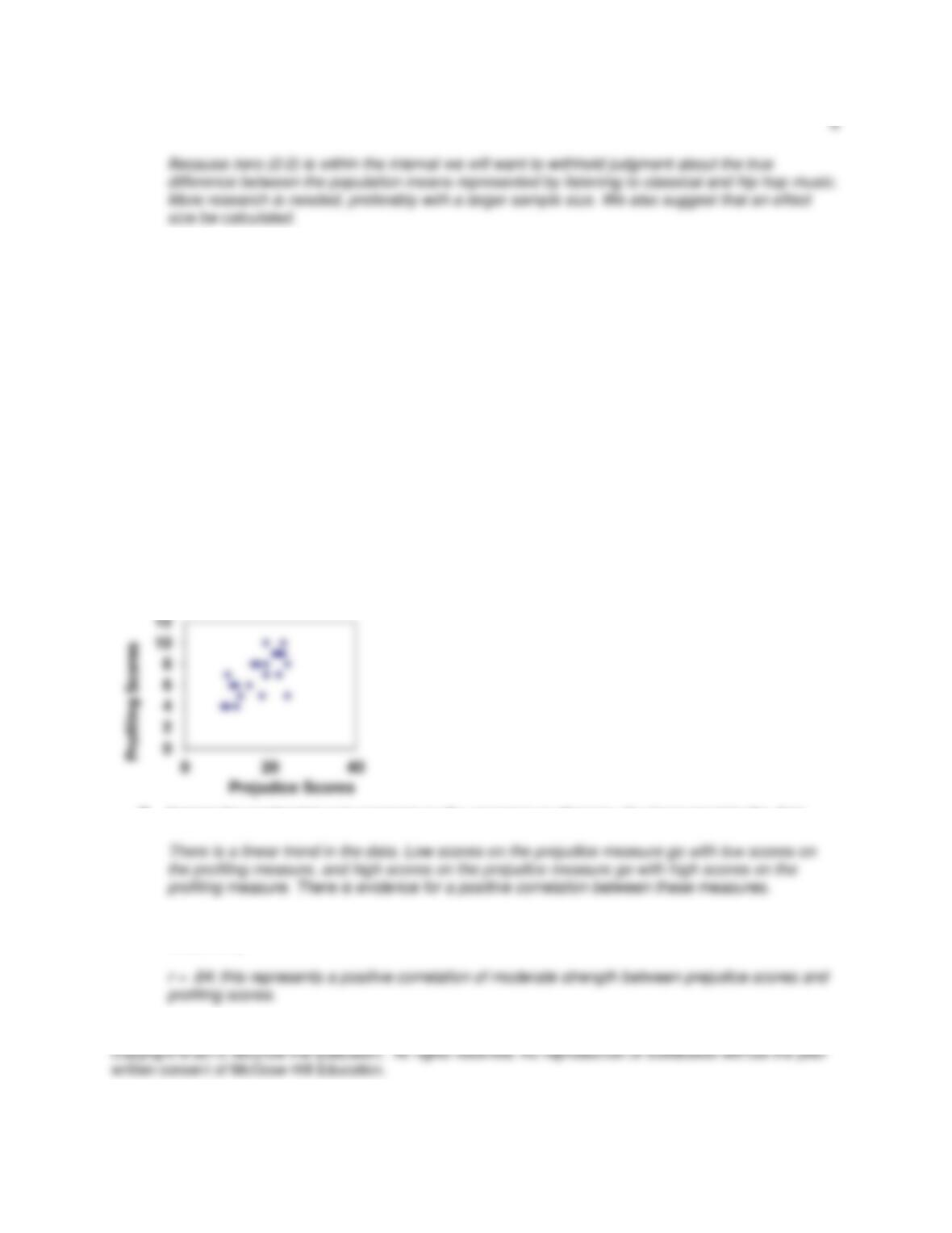
A. Calculate the means for each condition. What trend do you see in the comparison of means?
B. Calculate the estimated standard error of the difference scores.
C. Find the 95% confidence interval for the difference between the two means in this repeated
measures design.
D. State a conclusion regarding the effect of type of music on performance given the analysis of
these results.
9
causes people to support racial profiling by law enforcement agencies. Comment on this
conclusion based on what you know about the nature of correlational evidence.
ISSUES AND PROBLEMS FOR CLASS DISCUSSION
Presented below are suggestions and guides for in-class activities that allow students to think critically
about Chapter 11 concepts.
1. Using Confidence Intervals to Confirm What the Data Reveal
1. The width of the confidence interval indicates how precise is the estimation of the population
means.
2. If two intervals overlap, we know for sure that the population means are the same.
False. Some would argue that the population means are never exactly the same. However, more
3. The odds are 95% that the true population mean falls in each interval.
False. Students may be reminded of the analogy of tossing rings to surround a stake. The
contain the population mean within the interval).
4. If two intervals do not overlap, there is a 95% probability that the population means differ.
10
5. If two intervals do not overlap, we have good evidence that the population means differ.
difference between the means.
2. Examining Correlational Evidence
Students should be reminded that the topic of correlation was discussed in Chapters 2, 4, and 5. The
instructor will find exercises for students when “Examining Correlational Evidence” among the
instructor’s resources provided for Chapter 2.
LEARNING BY DOING RESEARCH
1. Investigating students’ attitudes on an issue of importance to them is a relatively easy task for a
research methods class (e.g., see Chapter 5, Survey Research.) A class activity could require each
member of a class to conduct a brief survey of a (nonprobability) sample of students. The data for all
members of the class could be pooled to yield a rather large sample size. Topics related to local
issues such as student happiness, food service, the fraternity/sorority system, athletics, parking,
computer facilities, tuition costs, and similar issues, may be of interest to students, or students may
choose a topic with more broad social relevance. Use of a 7-point or 10-point scale for responses to
questions about these topics will make for manageable data for analysis. Students can then be asked
to go through the three stages of data analysis for making inferences about a single population mean.
A. Getting to know the data (inspecting data based on a stem-and-leaf display)
B. Summarizing the data (finding measures of central tendency and dispersion)
C. Confirming what the data reveal (by calculating a confidence interval for a single mean)
2. Students may be asked to write a brief summary of results using APA format (see Chapter 13) based
on data from a survey when confidence intervals are used to confirm what the data mean.
3. Exercises providing data for analysis when comparing two means can be designed using suggestions
for research found in Chapter 6 and 7 and in the instructor’s resource material for Chapters 6 and 7.
4. Data for correlational analyses and interpretation can be generated based on ideas found in Chapter
5 or from responses incorporated as part of a survey (see Activity 1).
INSTRUCTOR’S LECTURE/DISCUSSION AIDS
The following pages reproduce content from Chapter 11 and may be used to facilitate lecture or
discussion.

1. Data Analysis: This page describes the three stages of data analysis, the analysis story, and
computer-assisted data analysis.
2. Stage 1: Get to Know the Data: The first stage of data analysis is described on this page.
3. Stage 2: Summarize the Data: This page describes statistics from the second stage of data analysis.
4-5. Stage 3: Confirm What the Data Reveal: These two pages illustrate the steps for computing
confidence intervals.
6. Interpreting Confidence Intervals: Basic guidelines for interpreting confidence intervals are described
on this page.
7. Data Analysis for Correlational Studies: This page identifies key points regarding correlational
analysis.

12
Data Analysis
• Get to know the data
▪ Inspect data carefully, identify errors in the data, consider whether the
data make sense
• Summarize the data
▪ Use descriptive statistics (central tendency, variability) and graphical
displays of data
• Confirm what the data reveal
▪ Inferential statistics
▪ Decide whether the data support a claim about behavior
• The analysis story
▪ After data analysis, construct a coherent narrative to
o Explain the findings
o Counter opposing interpretations
o Justify conclusions
▪ APA-style research manuscript
o Standard format in psychology
▪ Conference presentations
• Computer-assisted data analysis
▪ Statistical software and computers used to analyze data
▪ Need good knowledge of statistics and research methods
o to use software
o to interpret output of analyses

13
Stage 1: Get to Know the Data
$ Examine general features of the data, “clean” the data as necessary
$ Check for errors such as missing or impossible values, outliers
$ Stem-and-leaf display to visualize features of the data and identify
outliers
$ Good data descriptions include numerical, pictorial/graphical, and verbal
summaries

14
Stage 2: Summarize the Data
• Central tendency
▪ Mean (M) or arithmetic average
▪ Median (Md): Middle point of frequency distribution (score that splits
distribution in half)
▪ Mode: Most frequent score in distribution
• Variability or dispersion
▪ Range: Difference between highest and lowest scores in distribution
▪ Standard deviation (SD or s): How far, on average, a score (X) is
from the mean
∑(X – M)2
s = N – 1
▪ Variance (s2): square of the standard deviation
• Estimated standard error of the mean s
sM = √N
▪ Standard deviation of the theoretical sampling distribution of means
▪ Measures how well the sample mean estimates the population mean
▪ Small values of sM indicate good estimate
• Measures of effect size
▪ Information about strength of relationship between IV and DV
▪ Not affected by sample size
▪ Cohen’s d: difference between
2 sample means (e.g., treatment, control)
divided by the population standard deviation (σ)
M1 − M2 (n1 − 1)s12 + (n2 − 1)s22
d = σ σ = N
▪ Guidelines for interpreting Cohen’s d
small effect: d = .20 medium effect: d = .50 large effect: d = .80

15
Stage 3: Confirm What the Data Reveal
• Construct a Confidence Interval (CI) for the population parameter
• Confidence Interval for population mean
▪ Range of values which we state with a certain degree of confidence
includes the population mean
o Typically use 95% or 99% confidence (probability)
▪ Use sample mean (M) to estimate population mean
▪ Compute estimated standard error of sampling mean (sM)
• Formulas
upper limit of 95% CI: M + [t.05][sM] where t.05 = value of t-statistic
with N − 1 df, α = .05
lower limit of 95% CI: M − [t.05][sM]
• Example
Suppose 30 students take a brief intelligence test.
Results: M = 115, SD = 14
▪ Is 115 a good estimate of the mean for the population from which the
sample was drawn?
▪ sM = 2.55, critical value of t with 29 df, α = .05: t = 2.04
▪ Upper limit: 115 + [2.04][2.55] = 120.2
▪ Lower limit: 115 − [2.04][2.55] = 109.8
▪ We can state with 95% probability that the interval 109.8 to 120.2
contains the true population mean.
▪ The narrower the interval, the better the estimate
▪ Increasing the sample size improves the estimate.

16
Stage 3: Confirm What the Data Reveal, continued
• Confidence Interval for the difference between two means
▪ Similar procedure
▪ Substitute difference between two means for single mean
▪ Use estimated standard error for the difference between two means
sM1 – M2 = (n1 – 1)s12 + (n2 – 1)s22 1 + 1
n1 + n2 – 2 n1 n2
▪ This CI provides information about effect of IV with two conditions
▪ Formula: CI (95%) = (M1 − M2) ± t(.05)(sM1 − M2)
• Example
Suppose a treatment is designed to improve memory.
DV is correct recall on a memory test.
Treatment group: M = 64.04, s = 12.27, n = 26
Control group: M = 45.58, s = 10.46, n = 26
Difference between Means: 18.46 sM1 − M2 = 3.16
Critical value of t at α = .05, df = 50: t = 2.009
CI (.95) = 18.46 ± (2.009)(3.16)
upper limit: 18.46 + 6.35 = 24.81
lower limit: 18.46 − 6.35 = 12.11
▪ Conclusion: There is a .95 probability that the interval, 12.11 to 24.81,
contains the true population difference between the treatment and
control groups.
Mean memory performance, as measure by this test, can be
expected to improve by the amount indicated by the CI when this
treatment is implemented.

17
Interpreting Confidence Intervals
• Guidelines for CIs for difference between two means
▪ Note whether the CI includes the value zero
▪ When zero is not included in the CI
o We become more confident that the population means differ.
o An effect of the IV is likely present.
▪ When zero is included in the CI
o We are uncertain about the effect of the IV.
o It’s possible the IV has zero effect.
• Guidelines for CIs when comparing several independent group means
▪ Compute CI for each mean
▪ Use pooled standard deviation for estimated standard error of the
mean
▪ If the CIs do not overlap
o We can be confident the population means differ.
▪ If the CIs overlap slightly
o We become uncertain and postpone judgment.
▪ If the CIs overlap such that a sample mean falls within the CI for
another group
o We conclude the population means do not differ.

18
Data Analysis for Correlational Studies
• Correlation
▪ When two different measures of the same people, events, or things
vary together
o Scores on one variable covary with scores on another variable
• Stage 1: Get to know the data
▪ Check data for errors, impossible values, outliers
• Stage 2: Summarize the data
▪ Draw scatterplot
o Magnitude of correlation shown by how well data points conform to
a straight line (linear trend)
o Direction of correlation shown by upward (positive) or downward
(negative) trend in data points
▪ Calculate correlation coefficient
o Magnitude: zero indicates no relationship, strength of correlation
increases as value approaches |1.0|
o Direction: Sign of coefficient indicates positive (+) or negative (−)
correlation
• Interpreting correlations
▪ When two variables are correlated
o Make predictions for each variable
o If we know score for X, predict Y (and vice versa)
▪ Cannot make causal inferences

19
▪ Compute confidence interval for population correlation, ρ (rho)
o Similar to CI for population mean, μ