Chapter 08 – Cost Estimation
8-36 Cost Estimation: High-Low method (30 min)
1.
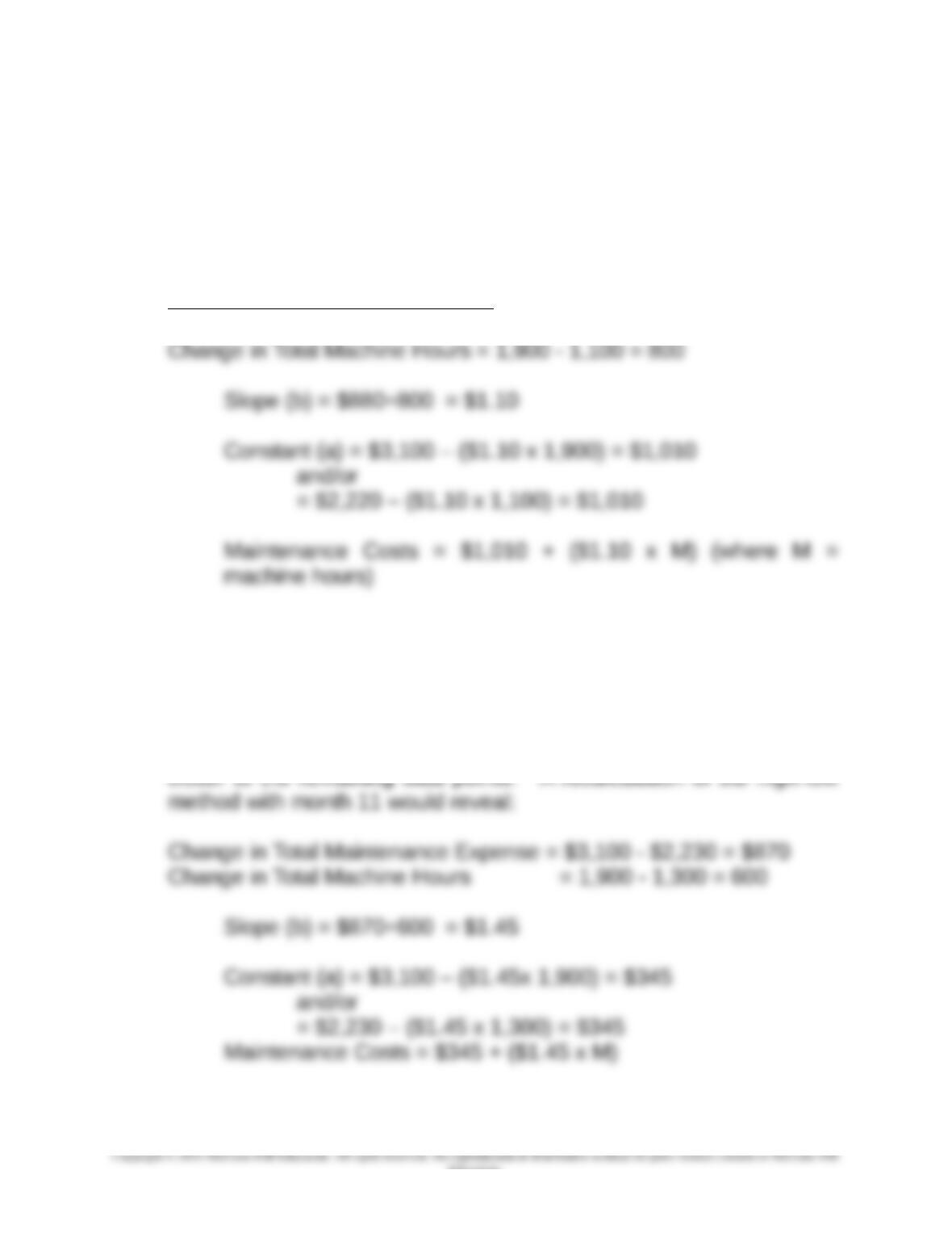
Model to fit: Maintenance Expense = a + b x M (machine hours)
The highest and lowest points are months 5 and 10, respectively.
The high-low method is as follows:
Change in Total Maintenance Expense = $3,100 – $2,220 = $880
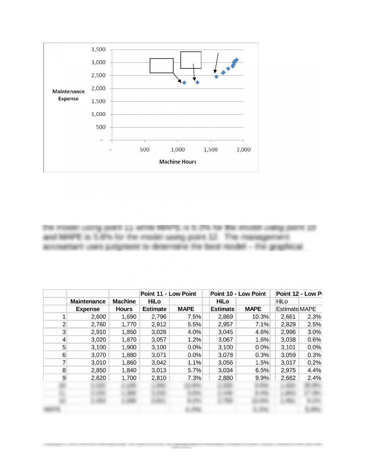
Note that an alternative solution might be preferred. On the basis of
a view of a graph of machine hours versus maintenance expense
(see below), it appears that the chosen lowest data point (month 10)
is not as representative of the relationships in the data as for month
11 (1,300 hours; $2,230). The point for month 10 is far to the left of
the remaining data points, while the point for month 11 is somewhat
8-21
Education.
Chapter 08 – Cost Estimation
8-36 (continued-1)
The graph of expense versus hours showing the point for month 10 to be
an outlier (to the far left of the graph). One might also argue that the point
for month 11 is also an outlier and that the data for month 12 (1,590 hours
and $2,450) should be used instead. The model using month 12 as the
lowest month would be:
8-22
Education.
12
Chapter 08 – Cost Estimation
8-36 (continued
-2)
2. The calculation of the mean absolute percentage error (MAPE) for each
of the two high low models discussed in part one shows that the model
based on point 11 is the superior model, under MAPE. MAPE is 4.4% for
view above leads to a choice of the model using point 12 while the MAPE
analysis leads to a choice of the model with point 11 as the low point.
8-23
Education.
11
10
Chapter 08 – Cost Estimation
8-37 The Gompertz Equation; Learning Curves (20 min)
1.
2. An exponential equation like the Gompertz equation could be used to
estimate the effect of employees working overtime on the production defect
rate, or it could be used to estimate the increase in maintenance cost as a
machine ages. These are examples of costs increasing at an exponential
rate as usage increases.
8-24
Education.
Chapter 08 – Cost Estimation
8-38 Regression and Utility Rates; Sustainability (20 min)
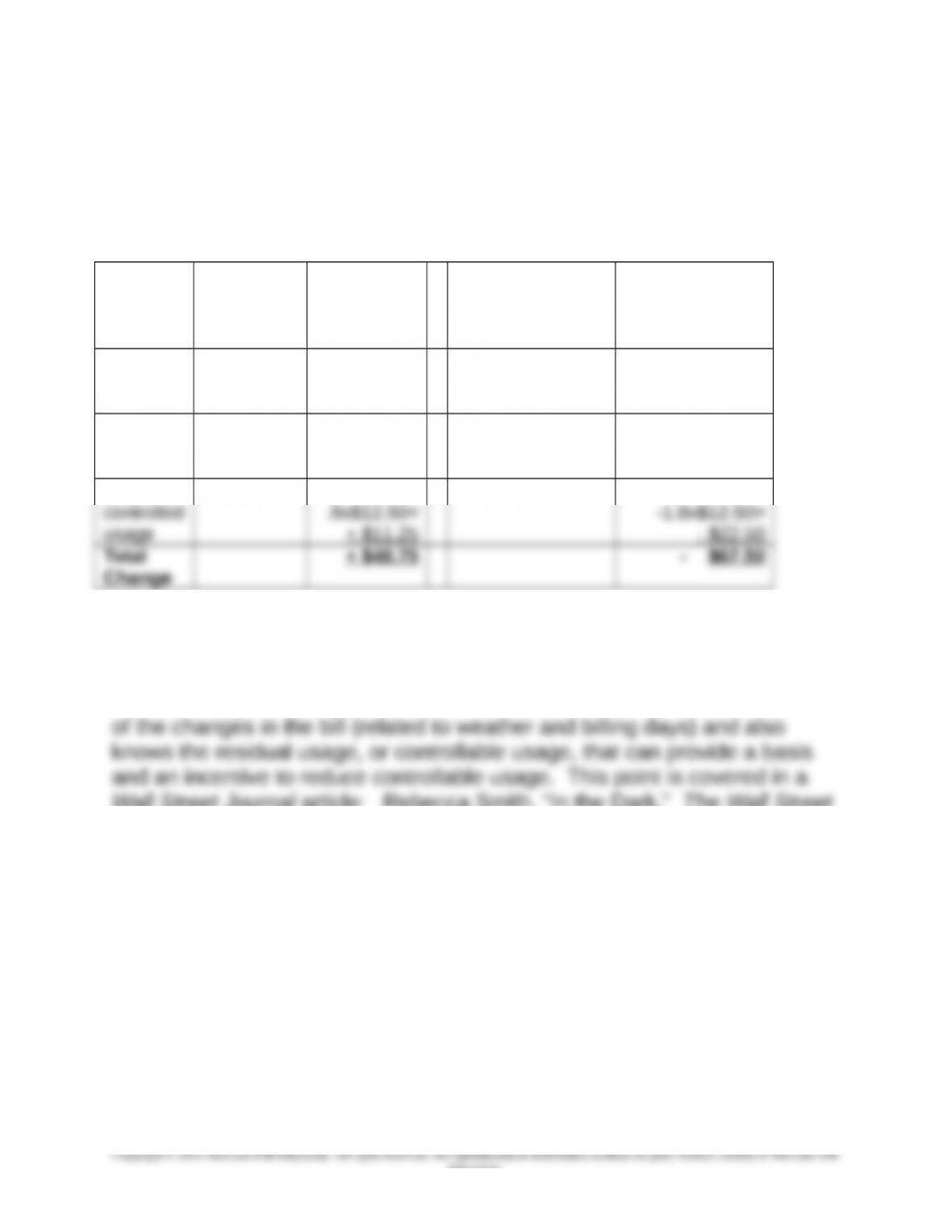
1. The calculations are as follows. The customer’s current bill was
$48.75 greater than last month’s bill, and $67.50 less than December
of the prior year.
Usage
Factors
Current
Month vs
Last
Month
$ Amount
Change
Current Month
vs this month
Last Year
$ Amount
Change
Weather 3 degrees
cooler;
+2.5MCF
2.5x$12.50
=
+ $31.25
8 degrees
warmer;
– 3.5MCF
-3.5x$12.50=
– $43.75
Number
of Billing
Days
5 more
days; +.5
MCF
.5x$12.50=
+ $6.25
1 less day; -0.1
MCF
-0.1x$12.50=
– $1.25
Customer
+.9 MCF
-1.8 MCF
Change
The above is based on an actual customer statement for a residence in
eastern Ohio.
The advantage of billing in this format is that the customer knows the cause
Wall Street Journal article: Rebecca Smith, “In the Dark,” The Wall Street
Journal, February 11, 2008, p R6.
2.
The Dominion billing system facilitates environmental sustainability by
showing each user a “report card” of their recent usage. The result is likely
to be an incentive for consumers to look for ways to reduce usage and
thereby reduce carbon-based emissions that lead to global warming.
8-25
Education.
Chapter 08 – Cost Estimation
8-39 Interpreting Regression Results (10 min)
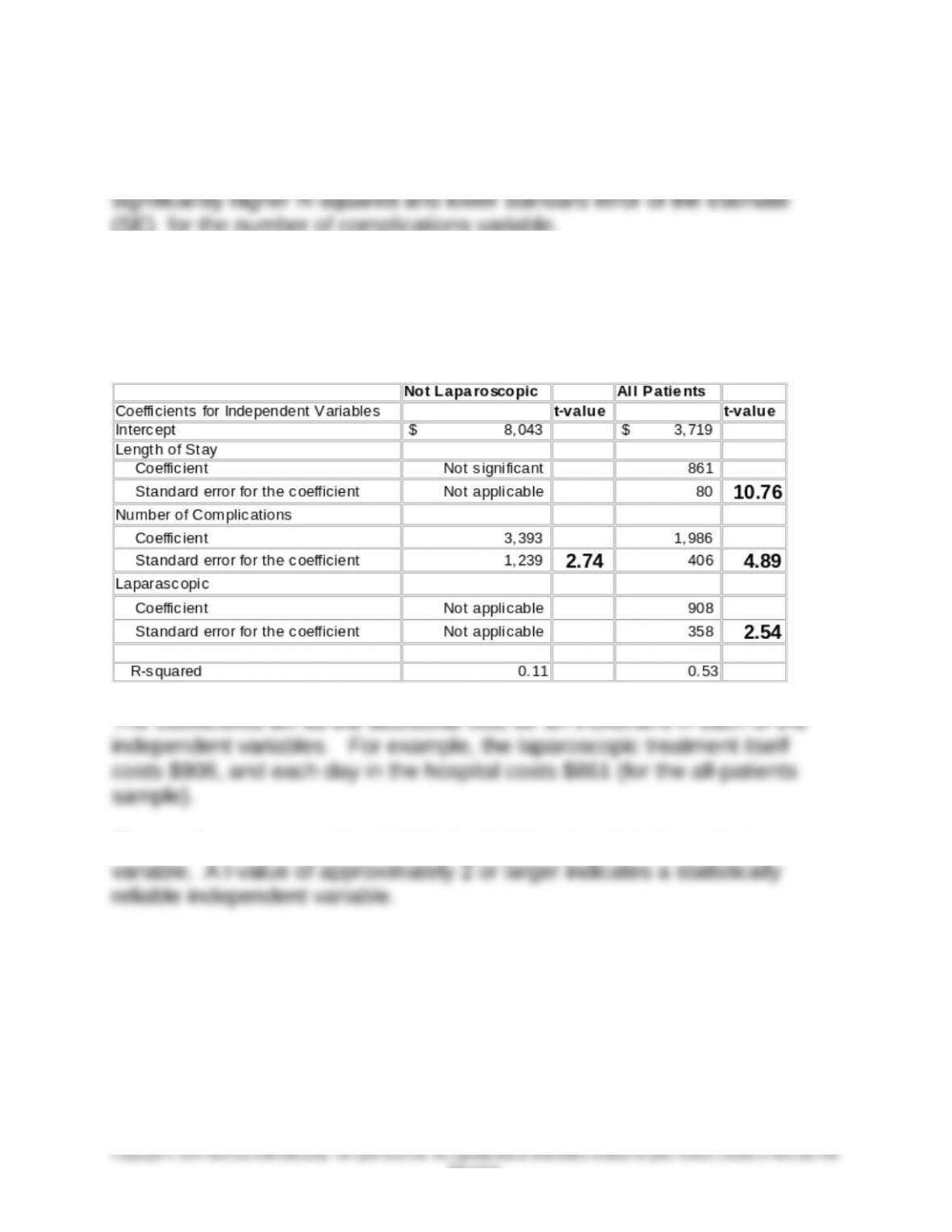
1. The estimated cost is:
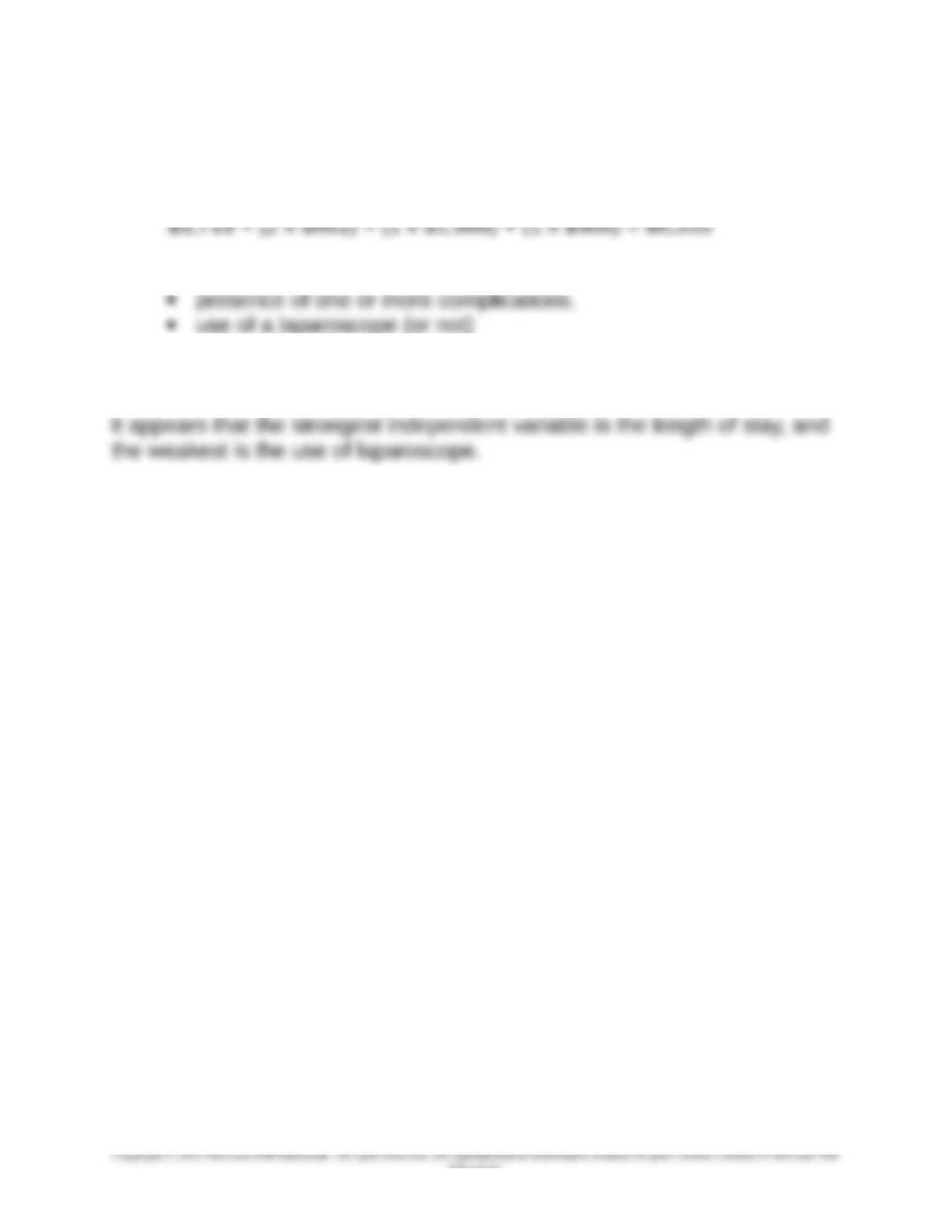
2. There are two dummy variables in this regression:
3. The model has a relatively low R-squared of only 53%, but all three
independent variables have good t-values (>2.0). Looking at the t-values,
The exercise is based on information from: “Hospital Costs of Uterine
Artery Embolization…” by M. Beinfeld, J. Bosch, and G. Gazette,
Academic Radiology, Nov 9, No. 11, November 2002, pp 1300-1304.
8-26
Education.
Chapter 08 – Cost Estimation
8-40 Analysis of Regression Results (10 min)
1. The laparoscopic regression has the better regression result, with a
(SE) for the number of complications variable.
2. The t-value is the ratio of the coefficient to the standard error of the
independent variable. The t-values are shown below.
The t-values measure the statistical reliability of each independent
8-27
Education.
Chapter 08 – Cost Estimation
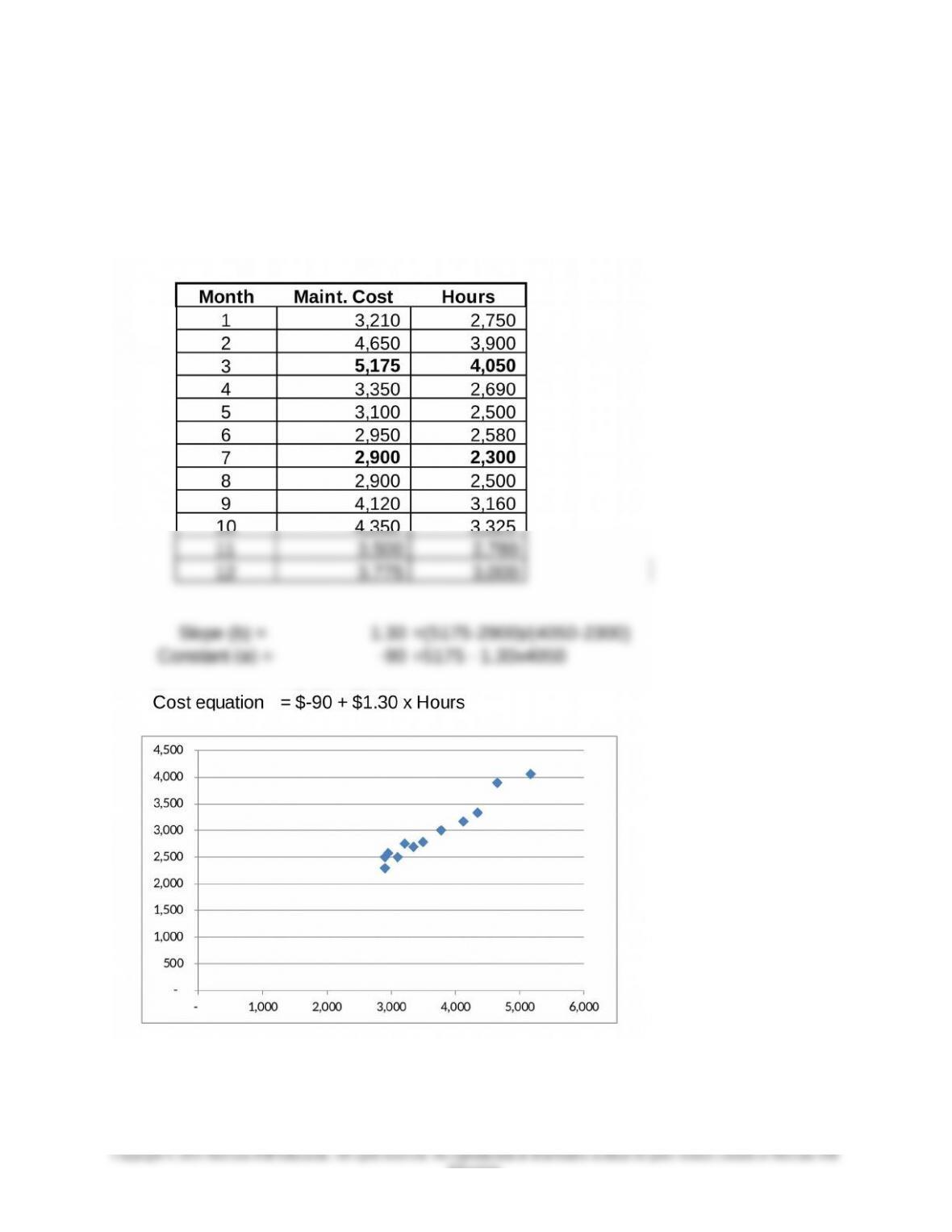
8-41 Cost Estimation; High-Low Method (15 min)
When months 3 and 7 are used for the high and low points respectively, the
High-Low method provides the cost equation: Cost = $-90 + $1.30 x hours.
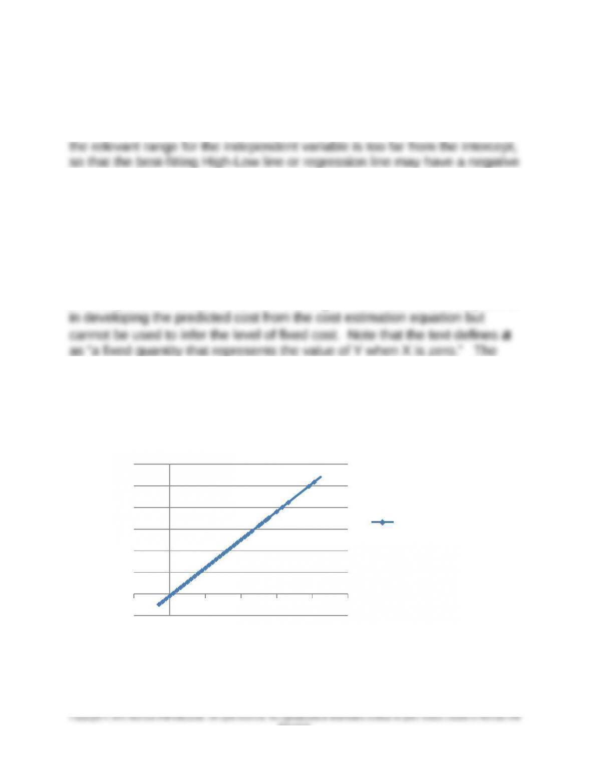
The graph below shows that the data is very linear; there are no outliers.
8-28
Education.
Chapter 08 – Cost Estimation
Exercise 8-41 (continued -1)
Note: the constant term in the solution is a negative number. This is a
good opportunity to explain to the students that a negative intercept term
can arise in a High-Low or a regression solution. The reason why is that
intercept. Chapter 3 included a discussion of the relevant range, with the
instruction that predictions of total cost should be limited to levels of the
independent variable that fall within the relevant range. This would be a
good time to remind the students of the concept of the relevant range and
how it applies to cost estimation. Wording to this effect is included on p
261 in the text.
This also reminds us that the value of a, the intercept, should not be
generally interpreted as fixed cost, especially when the relevant range of
the independent variable is far from the origin. The value of a is very useful
illustration below shows the high low line extended to the origin and the
negative intercept; the data below 2,300 hours is outside the relevant
range.
+
(1,000) – 1,000 2,000 3,000 4,000 5,000
(1,000)
–
1,000
2,000
3,000
4,000
5,000
6,000
Predicted Cost
Predicted Cost
Negative intercepts also appear in exercise 36 and in Problems 54,and 57.
8-29
Education.
Chapter 08 – Cost Estimation
PROBLEMS
8-42 Cost Estimation; High-Low Method and Regression (30 min)
1.
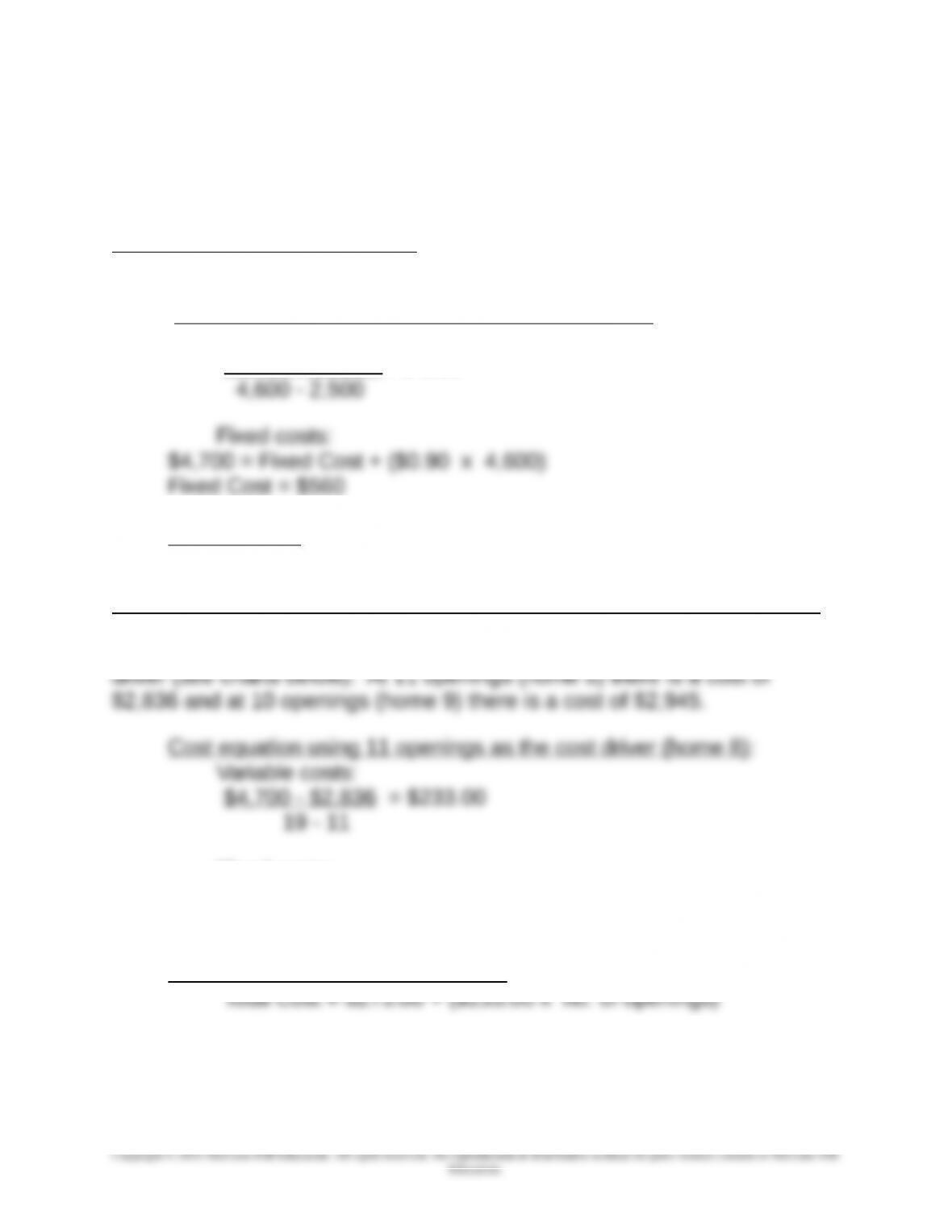
Analysis Based on Square Feet
The high point is Home 5 and the low point is Home 1
Cost equation using square feet as the cost driver:
Variable costs:
$4,700 – $2,810 = $ 0.90
Equation One: Total Cost = $560 + ($0.90 x no. of square feet)
Analysis Based on Openings: (high is home 5, low is either home 8 or 9)
There are two choices for the Low point when using openings for the cost
Fixed costs:
$4,700 = Fixed Cost + ($233.00 x 19)
Fixed Cost = $273.00
Equation for Home 8 (11 openings):
8-30