Chapter 17 – The Management and Control of Quality
17-37 (Continued)
The request by Sanchez is unethical because it would suppress information that
could influence an understanding of the results of operations by the company. Also,
by withholding information about the contingent liability, Sanchez is not
communicating information objectively.
2. Resolution of Ethical Conflict—the IMA Standards specify that when an individual
is faced with ethical issues, the individual should follow the policies established by
the organization to deal with (resolve) such conflicts. If these policies do not resolve
the ethical conflict, then the following courses of action are recommended:
The individual should discuss the issue with his/her immediate supervisor (except
If Stein is not able to achieve a satisfactory resolution of the matter, she should
submit the issue to the next management level. (Note: contact with levels above

Chapter 17 – The Management and Control of Quality
17-12
Education.

Chapter 17 – The Management and Control of Quality
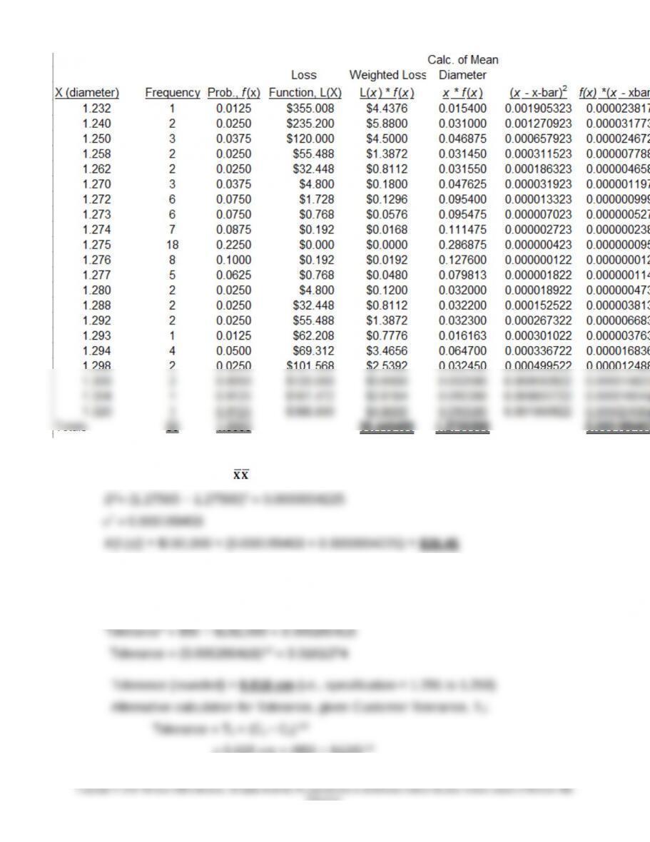
17-38 Taguchi Loss Function Analysis; Spreadsheet Application (50 Minutes)
1. k = Total quality cost ÷ (Tolerance allowed)2 = ($50 + $70) ÷ (0.025)2 = $192,000
17-13
Chapter 17 – The Management and Control of Quality
17-38 (Continued)
Mean actual diameter, = 1.2756500
2. Allowed diameter tolerance:
Repair Cost = k × (Tolerance) 2
$50 = $192,000 × (Tolerance)2
= 0.025 cm × ($50 ÷ $120)1/2
17-15
Education.

Chapter 17 – The Management and Control of Quality
= 0.025 cm × 0.645497 = 0.016 cm (rounded)
Note: An Excel spreadsheet solution file for this Problem is embedded in this document.
You can open the spreadsheet “object” that follows by doing the following:
1. Right click anywhere in the worksheet area below.
2. Select “worksheet object” and then select “Open.”
3. To return to the Word document, select “File” and then “Close and return to…”
while you are in the spreadsheet mode. The screen should then return you to the
Word document.
Ex. 17-38 7e.xlsx

Chapter 17 – The Management and Control of Quality
17-39 Six-Sigma Interpretation; Spreadsheet Application (20 minutes)
Sigma One-Tailed Two-Tailed Errors (Defects)
Level Area 1
Area Per Million
1 0.158655254 0.317310508 317,310.51
1Excel formula: = 1 − NORMSDIST(n), where n = sigma level (1, 2, …)
The preceding data indicate suggest a common misconception regarding the quality
level assumed under Six Sigma. Only when a defect is defined as any deviation from
the targeted level of the attribute (i.e., only when the “tolerance” is zero) will the
above approach represent the maximum number of defects per million opportunities
for error. Note, for example, that the expected number of errors (defects) under Six
Sigma is approximately 2 per billion (when any deviation from target is considered a
defect).
In actual practice, based on initial experience by Motorola, the application of Six
Sigma allows some variation (drift) around the target value. That is, there is an
assumption that no process can be maintained in perfect control (i.e., no “drift” at
all). Thus, in practice, a drift of 1.5 standard deviations around the target value is
“allowed.” Any deviation beyond this allowable “drift” would be considered a defect or
out-of-control process.
What this means is that a revised formula is needed to calculate the defects per
million as the Six-Sigma methodology is applied in practice. According to Pyxdek
(http://www.qualitydigest.com/may01/html/sixsigma.html) the Excel formula (under
the assumption of an allowable drift of 1.5 sigma) is: 1000000*(1 − NORMSDIST(Z-
1.5)), where 1.5 = allowable drift (in standard deviations) and Z = Sigma level. For Z
= 6.0, the Excel formula returns: 3.398, the defect-per-million figure commonly, but
perhaps mistakenly, reported in the literature. (Also see, J. R. Evans and W. M.
Lindsay, The Management and Control of Quality, 6th ed. (South-Western, 2005),
Chapter 10.)
17-17
Education.
Chapter 17 – The Management and Control of Quality
17-40 Management Accounting’s Role in Six-Sigma (25 Minutes)
At the most general level, the management accountant (because of expertise in the
measurement process) should be included as a member of the cross-functional Six–
Sigma project team whose responsibility it is to focus on a particular business
process, improve that process, and then move on to another project. The role of the
management accountant on the project team can perhaps best be described within
the context of the five phases of the DMAIC approach to process improvement:
Define, Measure, Analyze, Improve, and Control.
In the define phase, management accountants, because they are in the best
position to observe and document waste and excessive costs, can help identify
opportunities that warrant Six–Sigma-type projects. As a follow-up, management
accountants can help in the project selection process by providing reliable data
regarding estimated costs (e.g., required resources degree of difficulty, chance of
success) and benefits (e.g., cost savings, customer impact, expected time for project
completion) associated with alternative projects under review. In other words, they
the project helps define and measure the factors that have the most influence on
process performance.
actually occur.
Finally, in the control phase, the management accountant can help in the
development of control tools such as audits and check sheets that can be used to
ensure sustainability of the process improvements implemented in the preceding
stage.
Source: F. Rudisill and D. Clary, “The Management Accountant’s Role in Six Sigma,”
Strategic Finance (November 2004), pp. 35-39.
17-18
Education.
Chapter 17 – The Management and Control of Quality
17-41 Applying Six–Sigma Principles to the Accounting Function (30 Minutes)
Perhaps the most fundamental step in the project is selection of an appropriate
cross-functional team, including a project champion (in this case, it was the CFO of
the organization) and a project leader (usually either a Green Belt or Black Belt).
One framework for the project management process is DMAIC (Design, Measure,
Analyze, Improve, and Control). In the present example, the DMAIC phases
consisted of the following stages:
The Define Stage—the project team developed a statement of the problem (“Too
many hours are being spent preparing quarter-end financial statements.”) and a
goals statement (“Reduce direct hours worked for 18 schedules from over 100 hours
to 26 hours.”). The latter was determined in consultation with the person primarily
schedules, 28 hours. Thus, the overall cycle-time reduction goal was approximately
84 hours!
The Analyze Stage—in this stage, the team created a “fish-bone” (i.e., “cause-and-
effect”) diagram to identify possible root causes of the excessive cycle time for
quarterly closings. Four primary causes were identified: (1) a high number of hours
were spent on the balance sheet schedules, (2) the E-Trans submissions were
compiled a list of actions that addressed the causes of the potential failure modes.
Implementing these actions resulted in substantial process improvements: in the first
quarter alone, the total cycle time of the process was reduced to 32 hours, slightly
above the 26-hour goal.
17-19
Education.

Chapter 17 – The Management and Control of Quality
17-41 (Continued)
The Control Stage—in a sense, the most important control-related decision
17-20
Education.
Chapter 17 – The Management and Control of Quality
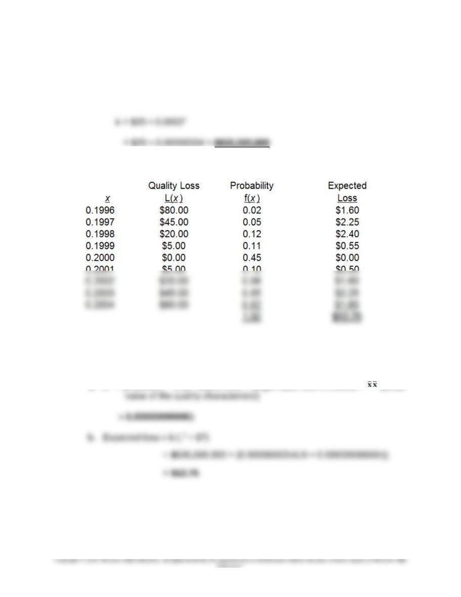
17-42 Taguchi Loss Function Analysis (50 Minutes)
1. Value of k, the cost coefficient, in the Taguchi Loss Function, L(x):
L(x) = k(x − T)2
2a & b. Expected Loss Using Taguchi Loss Function:
3. Expected Loss Using Variance Data (see table below), per Albrecht and Roth, “The
Measurement of Quality Costs: An Alternative Paradigm,” Accounting Horizons
(June 1992), pp. 15–27:
a. D2 = (0.199991 − 0.2)2, where 0.20 = target value and 0.199991 = (mean
17-21
Education.