Chapter 12 – Strategy and the Analysis of Capital Investments
12-34 Determining Cash Flows; Basic Capital Budgeting (15 minutes)
1. The after-tax cash flow from disposal of the old machinery = after-tax gain on sale =
($1,800 – $0) × (1 – t) = $1,800 × 0.60 = $1,080
2. The PV of after-tax operating cash savings = pre-tax operating cash savings × (1 –
12-21
Education.
Chapter 12 – Strategy and the Analysis of Capital Investments
12-35 Cash Flow Analysis; NPV; Spreadsheet Analysis (50 minutes)
1.
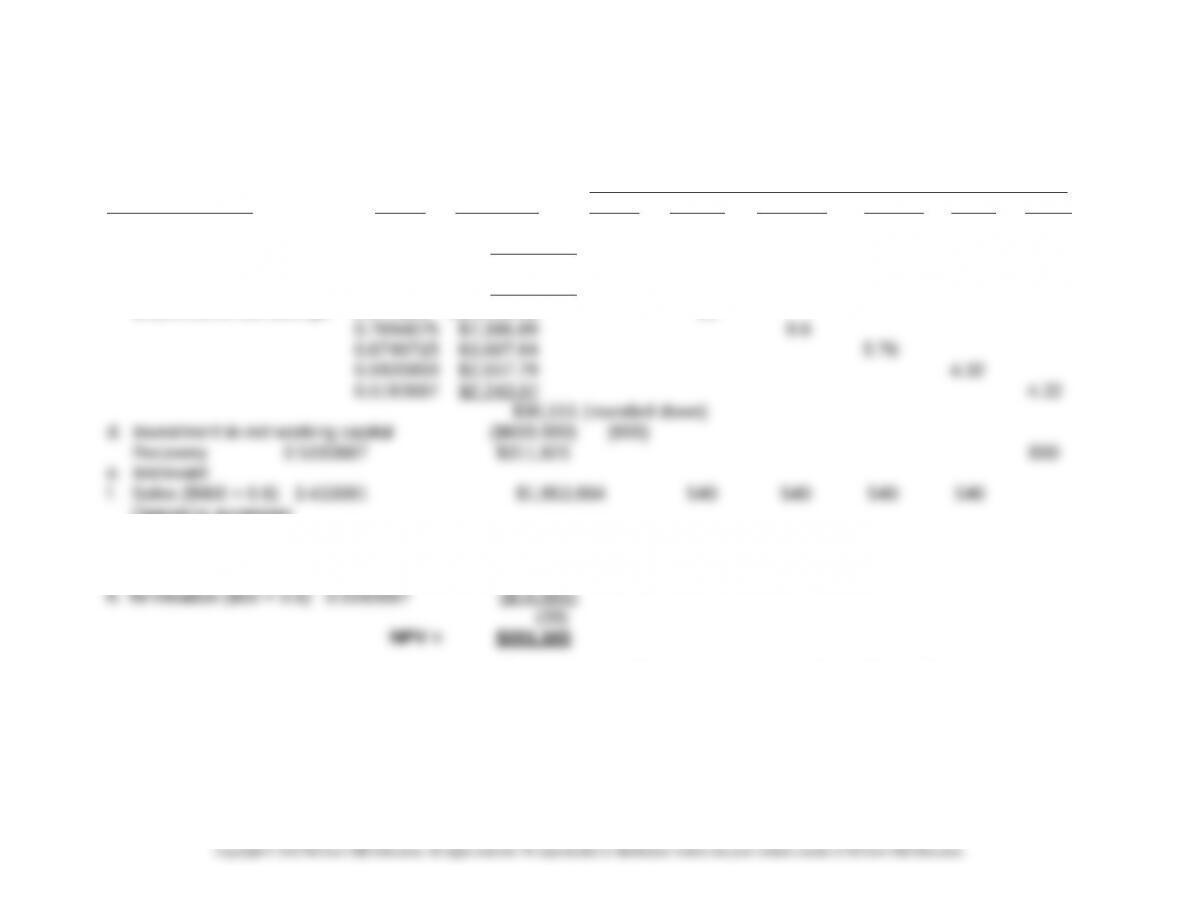
PV CASH FLOWS IN YEAR (in ‘000) )
Item & Description Factor PV 0 1 2 3 4 5
a. After-tax rent foregone
($5,000/mo. × 12 × 0.6) N/A ($128 ,931) 1(36) (36) (36) (36) (36)
b. All are irrelevant
c. Remodeling cost ($100 ,000) (100)
Depreciation tax savings2 0.877193 $14,035.09 16
Operating expenses
($500 × 0.6) 3.433081 ($1,029,924)
(300) (300) (300) (300) (300)
g. Sales Promotion ($100 × 0.6) ($60,000) (60)
Notes: When Excel is used, rather than the PV factors in text Tables 1 and 2, there will be a slight difference in
answers, due to rounding that takes place in the PV tables in the text. The PV factors presented above were calculated
using the following formula, for i = 1, 5: PV factori = (1/1.14i)
1Use the PV function in Excel to determine the PV of a stream of 60 monthly cash receipts ($3,000 per month, after-
tax). The appropriate formula is: =PV(0.14/12,60,3000).
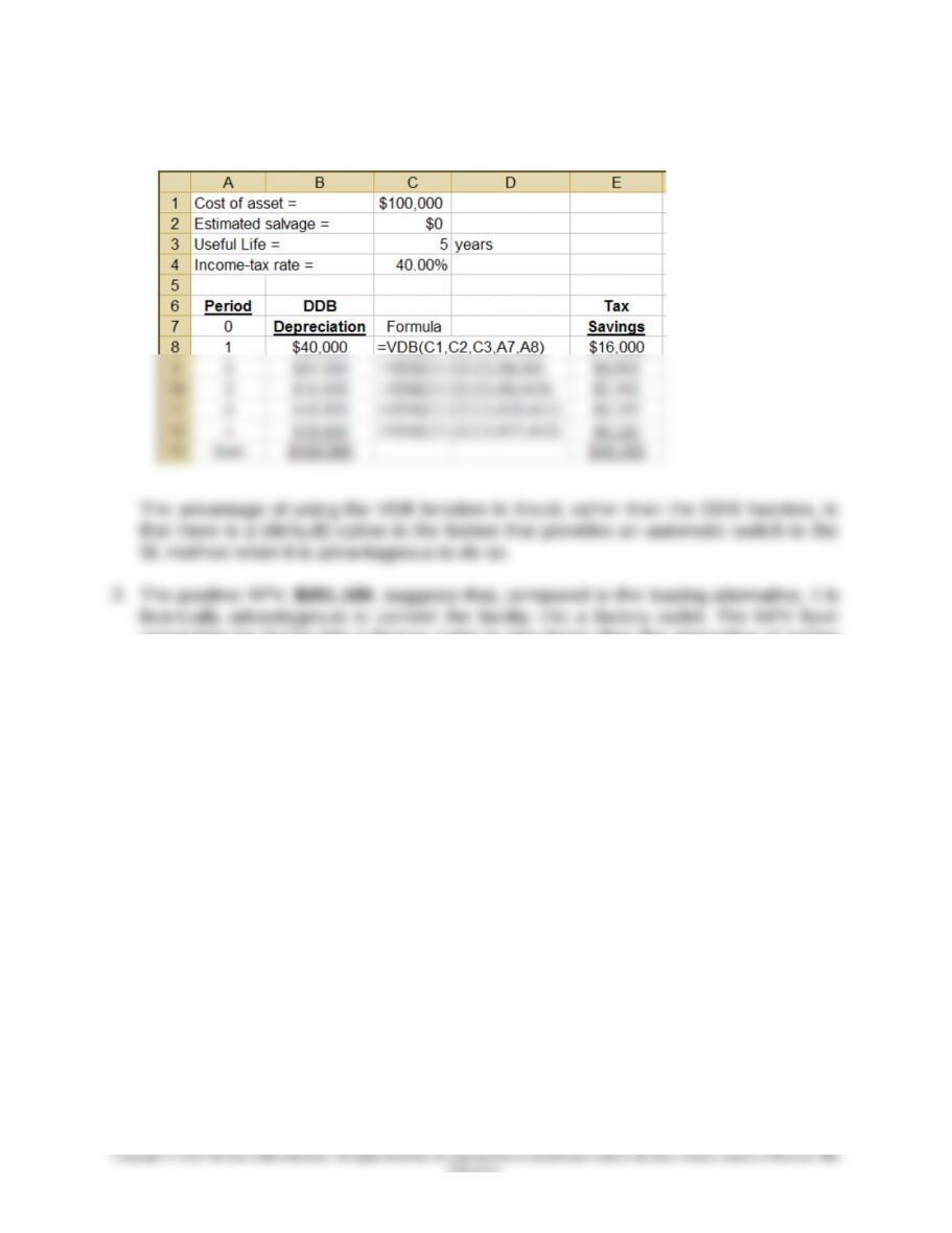
2Depreciation deductions found using the VDB function in Excel, as follows:
12-22

Chapter 12 – Strategy and the Analysis of Capital Investments
12-23
Chapter 12 – Strategy and the Analysis of Capital Investments
12-35 (Continued)
converting the facility into a factory outlet is also better than the alternative of selling
the warehouse for $200,000 (see item b).
12-24
Education.
Chapter 12 – Strategy and the Analysis of Capital Investments
12-36 Future and Present Values Using Excel (30 minutes)
A. To calculate future values, use the following Excel function:
FV(rate,nper,pmt, pv,type)
1. Between January 1, 1701 and December 31, 2015 there are 630 six-month
4. FV(0.08/2,12,0,-9500000000,0) = $15,209,806,076
B. To calculate present values, use the following Excel function:
1. For a stream of ten (10) end-of-year payments of $25,200,000 (ordinary
annuity) and a discount rate of 12%, we have:
2. If the first payment is received the day the contract is assigned (annuity due),
we have:
3. Given an income-tax rate of 45%, the after-tax cost of (1) above is:
Chapter 12 – Strategy and the Analysis of Capital Investments
12-37 NPV; Sensitivity Analysis (20 minutes)
1. NPV of proposed investment,15-year project life:
PV of after-tax cash inflows = $600,000 × 6.142 = $3,685,200
Initial investment outlay = 3,500,000
2. We are given annual after-tax cash inflows of $600,000 and an initial
investment outlay of $3,500,000. To generate an IRR of exactly 14.00%, the
following must hold:
PV of Future Cash Inflows = Initial Investment Outlay
$600,000 × An,14% = $3,500,000
Thus, we need to solve for the particular n that balances the preceding
equation. An, 14% = $3,500,000 ÷ $600,000 = 5.833. This annuity factor, at 14%,
In the present case, the annuity factor = 5.83333 and r = 0.14. Thus, we have
5.83333 = [1 ÷ 0.14] × [1 – [1 ÷ (1.14)n]]
(2) Next, subtract 1 from both sides, to yield:
-0.1833338 = – 1 ÷ (1.14)n
12-26
Chapter 12 – Strategy and the Analysis of Capital Investments
12-37 (Continued)
(3) Multiply both sides by –1:
0.1833338 = 1 ÷ (1.14)n
(4) By rule of exponents (i.e., 1 ÷ xn = x-n), the right-hand side of the above
0.1833338 = 1.14-n
(6) Take the log of each side of (5), which gives us:
log 0.1833338 = log 1.14-n
12-27
Education.
Chapter 12 – Strategy and the Analysis of Capital Investments
12-38 Uneven Cash Flows; NPV; Sensitivity Analysis (35 minutes)
1. Present value of net cash inflows:
Year 1 -0-
Year 2 $1,000,000 × 0.797 = $ 797,000
Year 3 $1,000,000 × 0.712 = 712,000
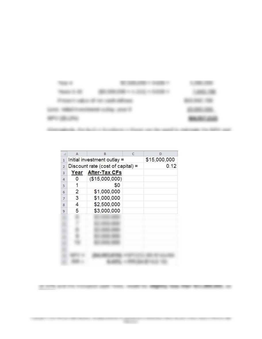
Alternatively, the built-in functions in Excel can be used to estimate the NPV and
the IRR of this project, as follows (Note: the slight difference in answers is due to
rounding—that is, the PV factors in the Tables have been rounded):
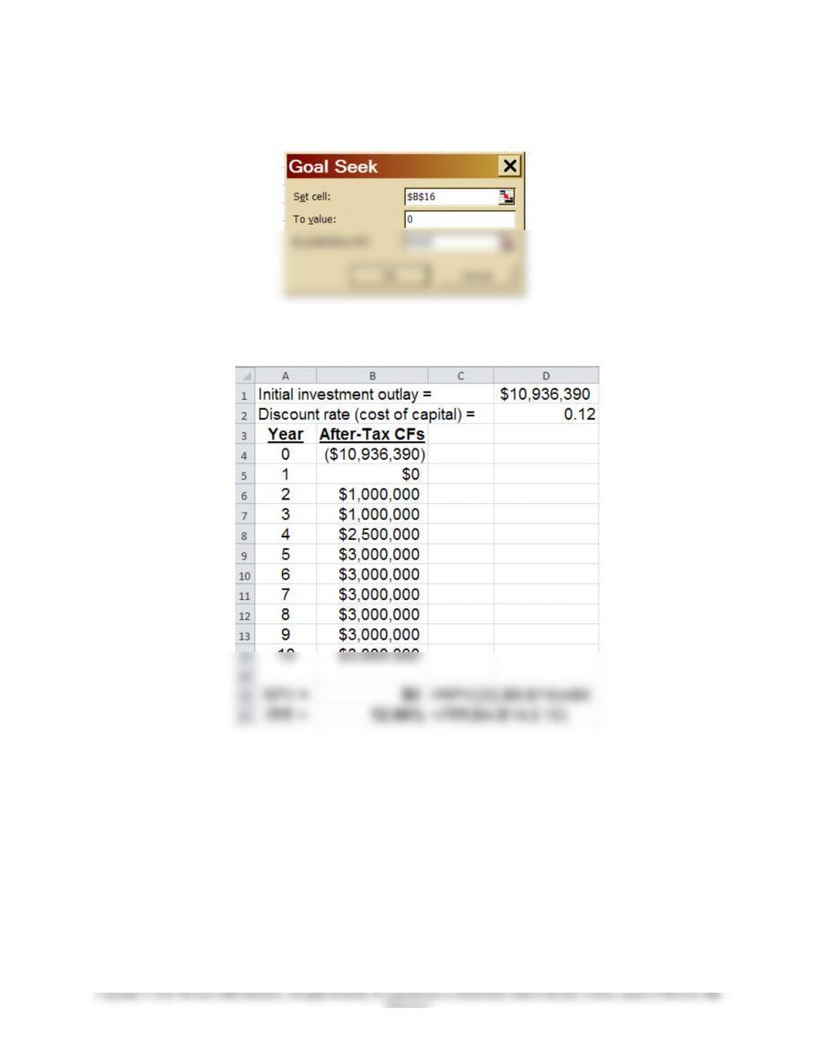
2. The maximum purchase price the seller would be willing to offer, given a discount rate
follows:
12-28
Chapter 12 – Strategy and the Analysis of Capital Investments
12-38 (Continued)
After executing Goal Seek, the following result is obtained for cell D1:
12-29
Education.
Chapter 12 – Strategy and the Analysis of Capital Investments
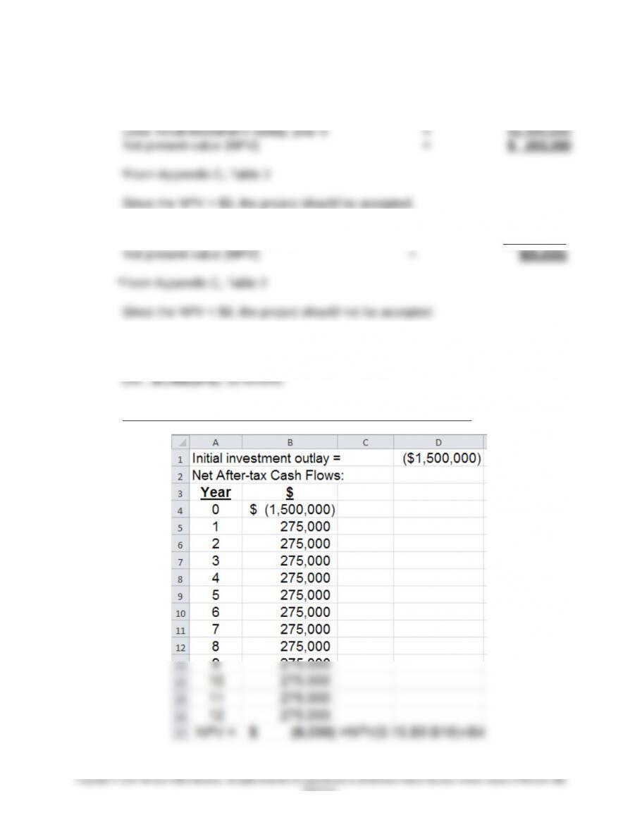
12-39 Risk and NPV; Sensitivity Analysis (45 minutes)
1. PV of future cash inflows: 12 years @ 12% = $275,000 × 6.194* = $1,703,350
2. PV of future cash inflows @ 15% = $275,000 × 5.421* = $1,490,775
Less: Investment outlay, year 0 = $1 ,500,000
3. The “break-even” initial investment outlay is the amount that would produce a
NPV = $0, given the annual after-tax flows of $275,000 and a discount rate of
15.00%. We can use Excel to solve, in two steps, for this “break-even” amount
Step 1: Estimate the Project’s NPV (compare with 2 above)
12-30
Education.