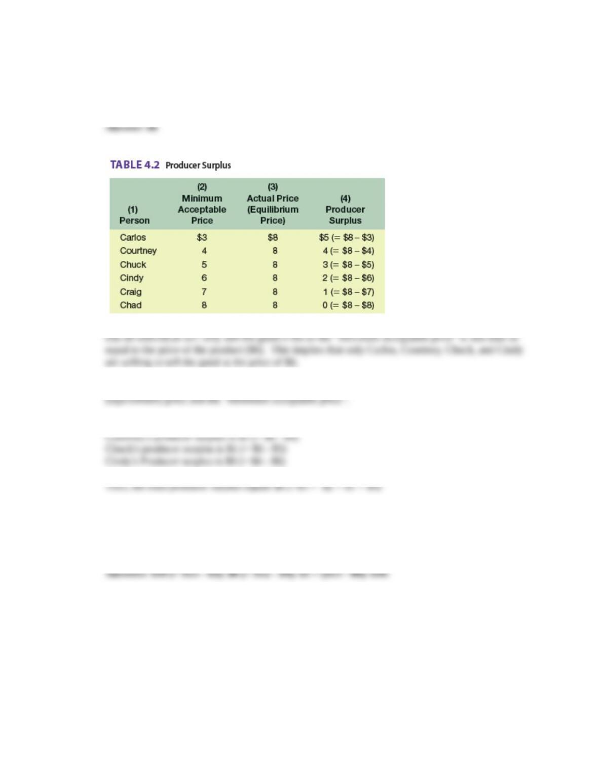
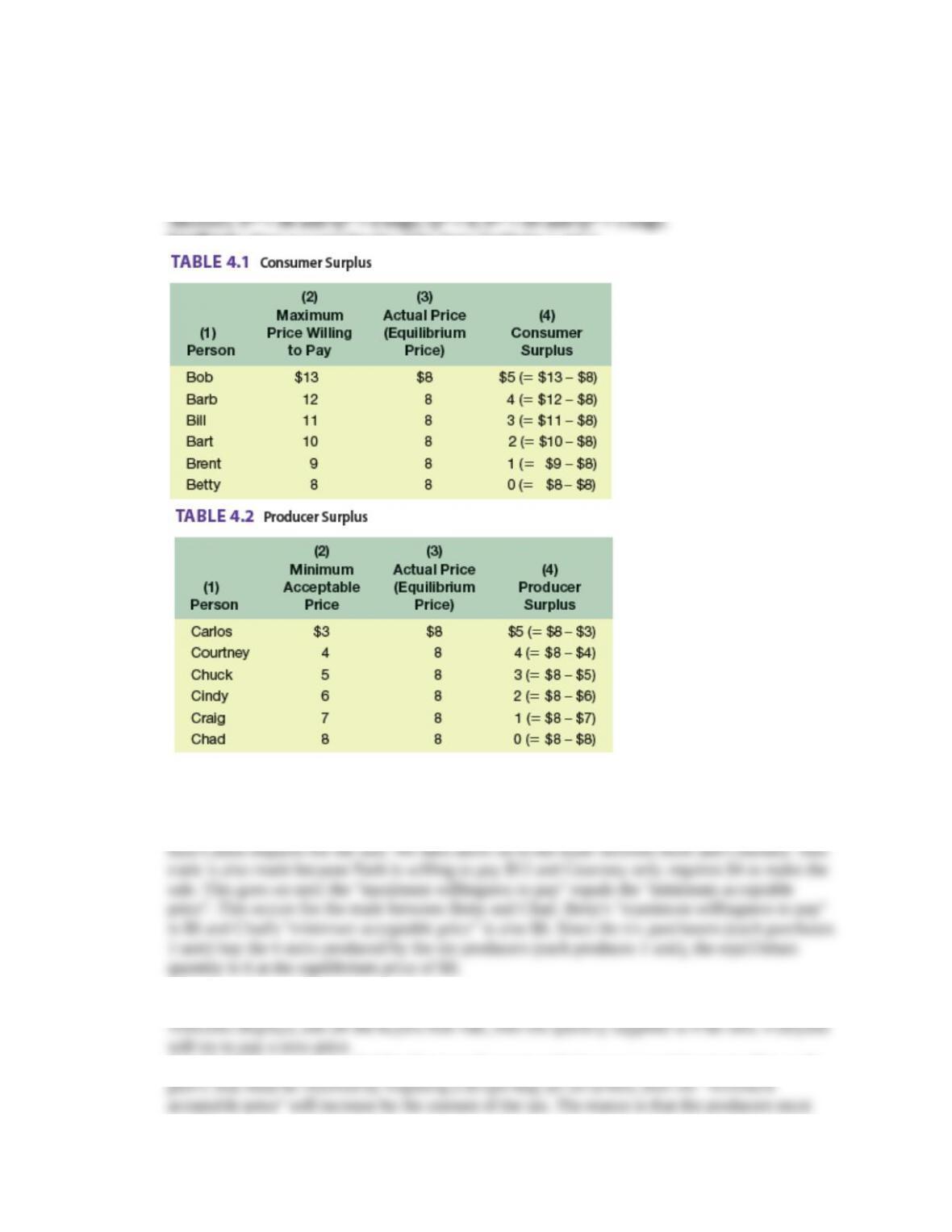
2. Refer to Table 4.2. If the six people listed in the table are the only producers in the market and the
equilibrium price is $6 (not the $8 shown), how much producer surplus will the market generate? LO2
Feedback: Consider the following table as an example:
Using the values above, and assuming an equilibrium price of $6 (not the $8 shown), we first note
Now we can calculate the producer surplus by adding up the difference between the actual
Carlos’s producer surplus is $3 (= $6 – $3)
3. Look at Tables 4.1 and 4.2 together. What is the total surplus if Bob buys a unit from Carlos? If Barb
buys a unit from Courtney? If Bob buys a unit from Chad? If you match up pairs of buyers and sellers so
as to maximize the total surplus of all transactions, what is the largest total surplus that can be achieved?
LO2
Feedback: Consider the following tables as an example:
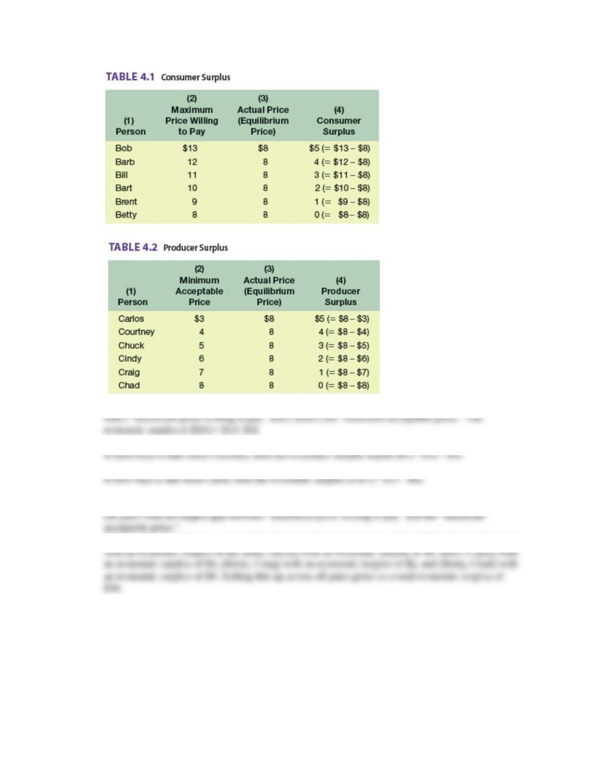
If Bob buys a unit of the good from Carlos, then the economic surplus is the difference between
If we match up buyers and sellers to maximize the total economic surplus then we need to choose
This implies the following pairs (Bob, Carlos) with an economic surplus of $10, (Barb, Courtney)
4. ADVANCED ANALYSIS Assume the following values for Figures 4.4a and 4.4b. Q1 = 20 bags. Q2 =
15 bags. Q3 = 27 bags. The market equilibrium price is $45 per bag. The price at a is $85 per bag. The
price at c is $5 per bag. The price at f is $59 per bag. The price at g is $31 per bag. Apply the formula for
the area of a triangle (Area = ½ x Base x Height) to answer the following questions. LO2
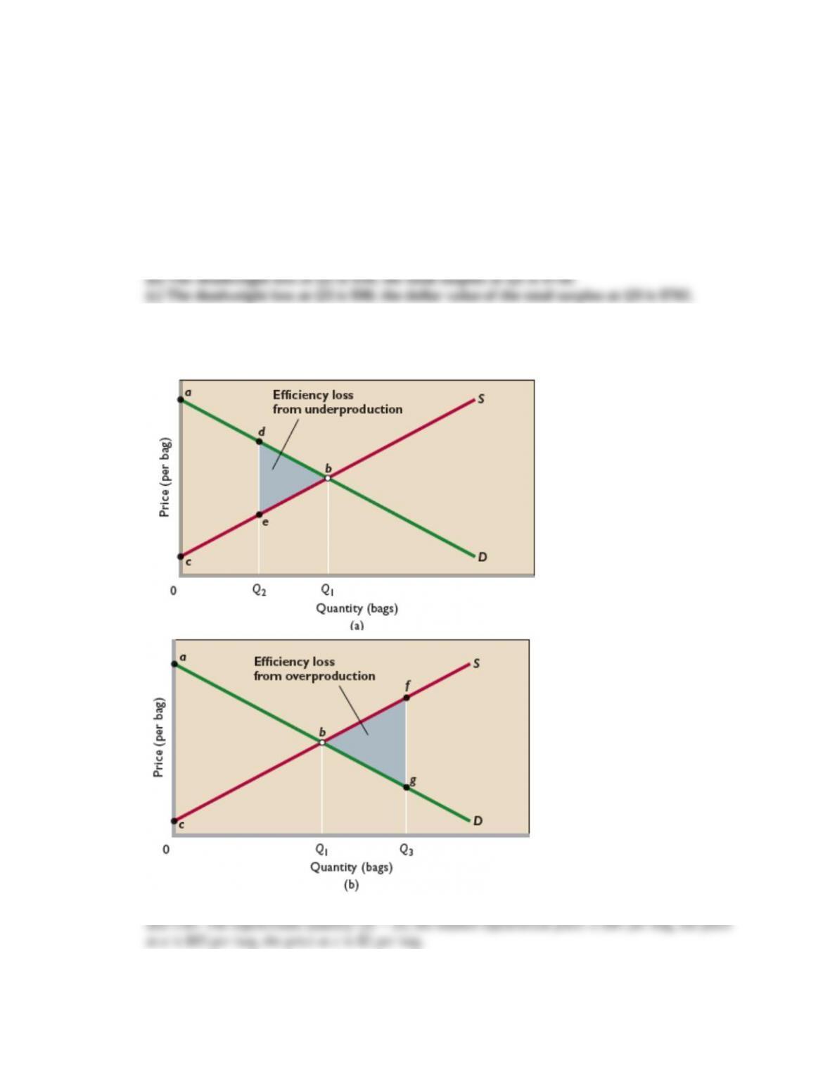
a. What is the dollar value of the total surplus (producer surplus plus consumer surplus) when the
allocatively efficient output level is being produced? How large is the dollar value of the consumer
surplus at that output level?
b. What is the dollar value of the deadweight loss when output level Q2 is being produced? What is the
total surplus when output level Q2 is being produced?
c. What is the dollar value of the deadweight loss when output level Q3 is produced? What is the dollar
value of the total surplus when output level Q3 is produced?
Answers:
(a) At output level Q1, total surplus is $800; consumer surplus at Q1 is $400.
Feedback: To answer this question, let us first find the mathematical representation of the supply
and demand schedules. To help us accomplish this objective we us the following figures.
Now consider the following values as an example. Assume the following values for Figures 5.4a
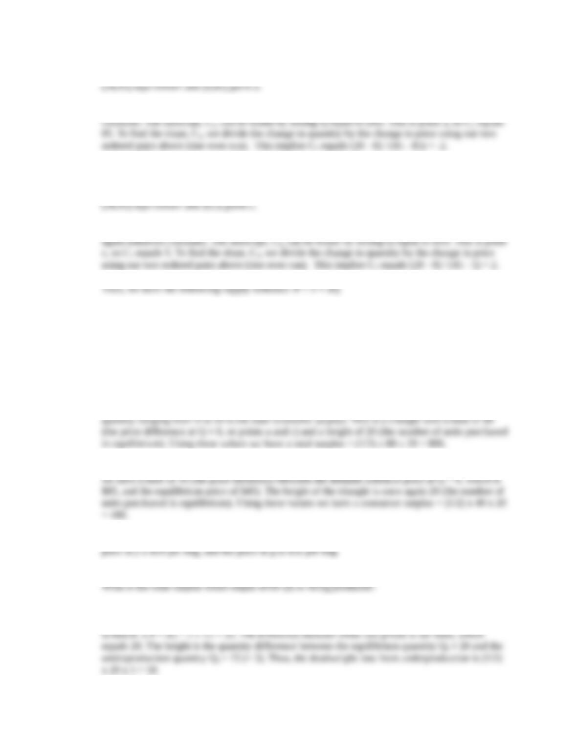
To derive the demand schedule (inverse demand schedule), we use the following ordered pairs:
We know the form of the demand schedule will be P=C1 + C2Q where C1 and C2 are unknown
Thus, we have the following demand schedule: P = 85 – 2Q
To derive the supply schedule (inverse supply schedule), we use the following ordered pairs:
We know the form of the supply schedule will also be P = C1 + C2Q where C1 and C2 are once
With these schedules we can now answer the following questions:
Part (a): What is the dollar value of the total surplus (producer surplus plus consumer surplus)
when the allocatively efficient output level is being produced? How large is the dollar value of
the consumer surplus at that output level?
To calculate total surplus we use the following formula for the area of a triangle (Area = ½ (Base
x Height)).
The area between the demand schedule P = 85 – 2Q and the supply schedule P = 5 + 2Q for the
The consumer surplus is the area between the demand curve and the equilibrium price line. Here
Consider the following additional values for the figures above: Q2 = 15 bags. Q3 = 27 bags, the
Part (b): What is the dollar value of the deadweight loss when output level Q2 is being produced?
The first thing we need to do is calculate the price at Q2 = 15 for the supply and demand
schedules. The price on the supply schedule is P = 5 + 2 x 15 = 35. The price on the demand
The total surplus can be found by subtracting the deadweight loss from the original total surplus
Part (c): What is the dollar value of the deadweight loss when output level Q3 is produced? What
is the dollar value of the total surplus when output level Q3 is produced?
Here we follow the same procedure. We are given the price at point f is $59 and the price at point
The total surplus can be found by subtracting the deadweight loss from the original total surplus
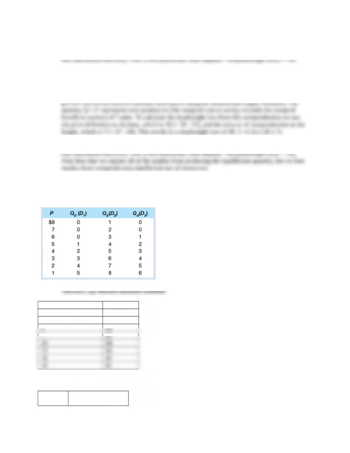
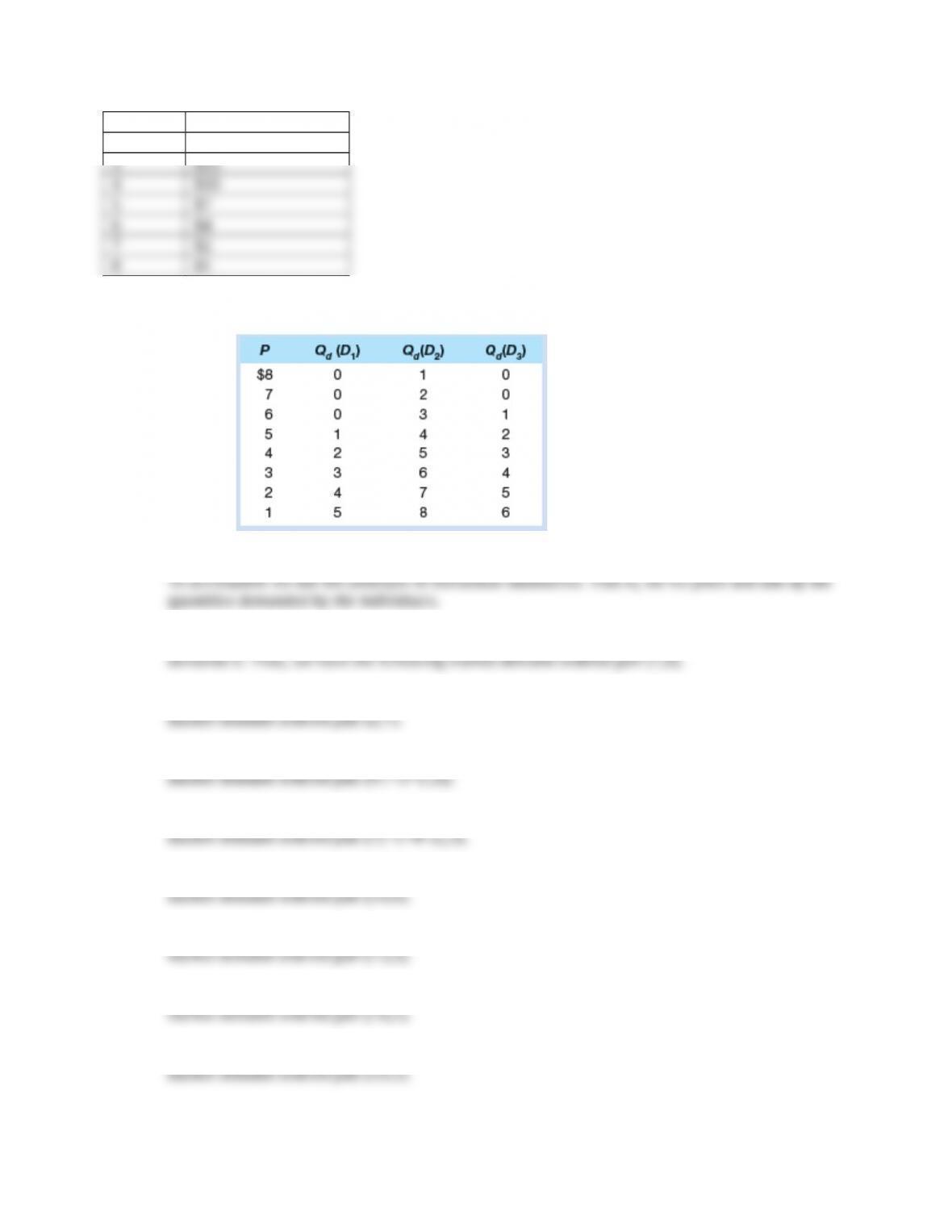
5. On the basis of the three individual demand schedules below, and assuming these three people are the
only ones in the society, determine (a) the market demand schedule on the assumption that the good is a
private good and (b) the collective demand schedule on the assumption that the good is a public good.
LO3
Quantity Demanded Price
1 $8
2 $7
(b) Collective demand schedule
Quantit
y
Amount Society is
Willing to Pay
1 $19
2 $16
Feedback: Consider the following table:
Part (a): Derive the market demand schedule on the assumption that the good is a private good.
At a price of $8: individual 1 (I1) demands 0, individual 2 (I2) demands 1, and individual 3 (I3)
At a price of $7: I1 demands 0, I2 demands 2, and I3 demands 0. Thus, we have the following
At a price of $6: I1 demands 0, I2 demands 3, and I3 demands 1. Thus, we have the following
At a price of $5: I1 demands 1, I2 demands 4, and I3 demands 2. Thus, we have the following
At a price of $4: I1 demands 2, I2 demands 5, and I3 demands 3. Thus, we have the following
At a price of $3: I1 demands 3, I2 demands 6, and I3 demands 4. Thus, we have the following
At a price of $2: I1 demands 4, I2 demands 7, and I3 demands 5. Thus, we have the following
At a price of $1: I1 demands 5, I2 demands 8, and I3 demands 6. Thus, we have the following
Part (b): Derive the collective demand schedule on the assumption that the good is a public good.
To accomplish we use the principle of vertical summation. That is, we fix quantity and add up the
price (willingness to pay) for the individuals. The logic here is that the individuals (society) can
pool resources to purchase a given quantity because this good will be shared (public good).
At the quantity 1: I1 is willing to pay $5, I2 is willing to pay $8, and I3 is willing to pay $6. Thus,
At the quantity 2: I1 is willing to pay $4, I2 is willing to pay $7, and I3 is willing to pay $5. Thus,
At the quantity 3: I1 is willing to pay $3, I2 is willing to pay $6, and I3 is willing to pay $4. Thus,
At the quantity 4: I1 is willing to pay $2, I2 is willing to pay $5, and I3 is willing to pay $3. Thus,
At the quantity 5: I1 is willing to pay $1, I2 is willing to pay $4, and I3 is willing to pay $2. Thus,
At the quantity 6: I1 is willing to pay $0, I2 is willing to pay $3, and I3 is willing to pay $1. Thus,
At the quantity 7: I1 is willing to pay $0, I2 is willing to pay $2, and I3 is willing to pay $0. Thus,
At the quantity 8: I1 is willing to pay $0, I2 is willing to pay $1, and I3 is willing to pay $0. Thus,
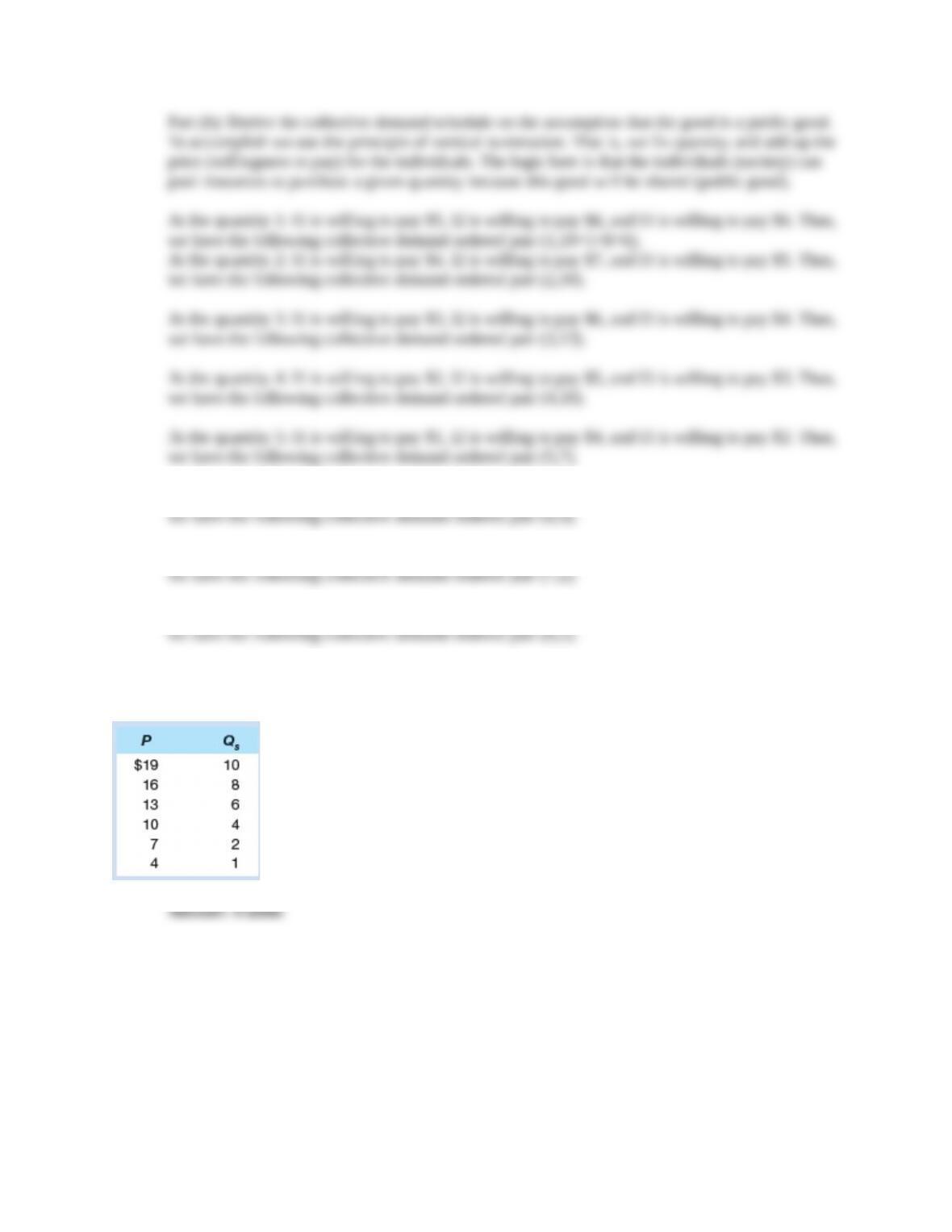
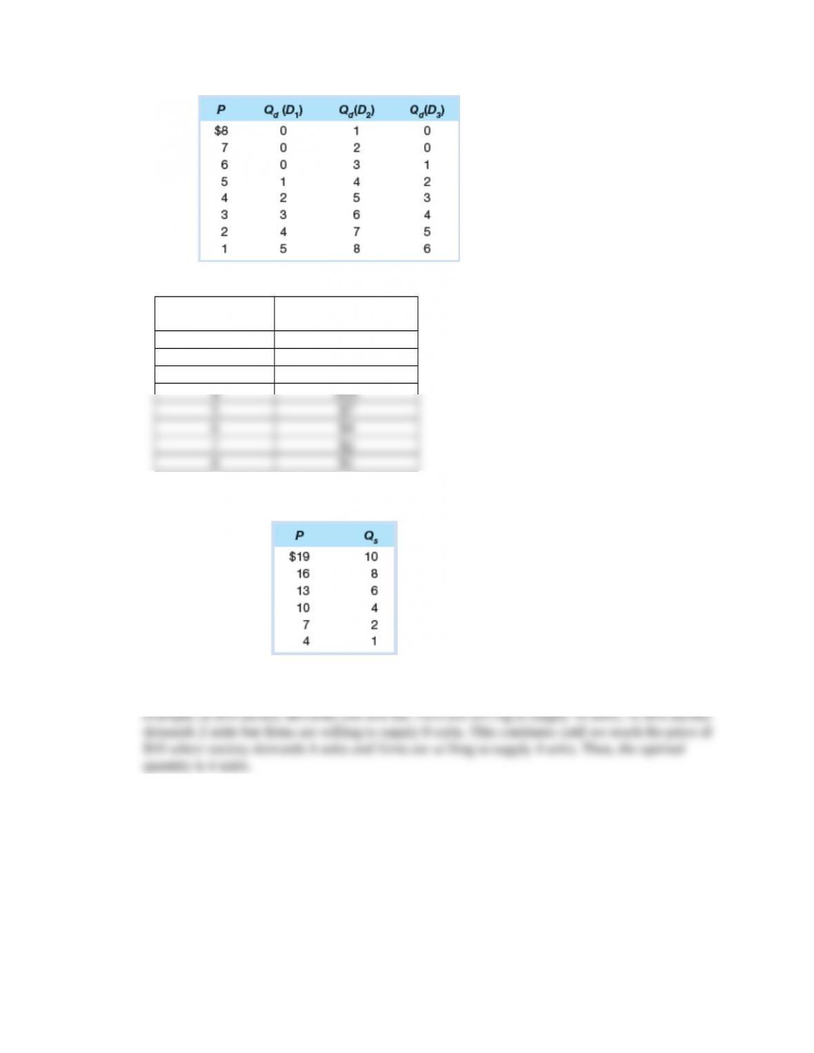
6. Use your demand schedule for a public good, determined in problem 5, and the following supply
schedule to ascertain the optimal quantity of this public good. LO3
Feedback: From the example table in problem 5, we calculated the collective demand schedule
from the individual demand schedules:
Collective Demand Schedule:
Quantity Price Society is
Willing to Pay
1 $19
2 $16
3 $13
Combining this collective demand schedule with the following supply schedule, we can
determine the optimal provision (quantity) of the public good.
The optimal quantity can be found by finding the price where the willingness to pay equals price
required by the firm to supply that last unit (basically the price that clears the market). For
7. Look at Tables 4.1 and 4.2, which show, respectively, the willingness to pay and willingness to accept
of buyers and seller of bags of oranges. For the following questions, assume that the equilibrium price and
quantity will depend on the indicated changes in supply and demand. Assume that the only market
participants are those listed by name in the two tables. LO4
a. What are the equilibrium price and quantity for the data displayed in the two tables?
b. What if instead of bags of oranges, the data in the two tables dealt with a public good like fireworks
displays. If all the buyers free ride, what will be the quantity supplied by private sellers?
c. Assume that we are back to talking about bags of oranges (a private good), but that the government has
decided that tossed orange peels impose a negative externality on the public that must be rectified by
imposing a $2-per-bag tax on sellers. What is the new equilibrium price and quantity? If the new
equilibrium quantity is the optimal quantity, by how many bags were oranges being overproduced before?
Feedback: Here we consider the tables from Problems 1 and 2.
Part (a): To determine the equilibrium price of oranges, we begin by comparing the highest
willingness to pay with the lowest minimum acceptable price. Bob is willing to pay $13 and
Carlos is willing to accept at minimum $3. This trade is made because Bob is willing to pay more
Part (b): If instead of bags of oranges, the data in the two tables dealt with a public good like
Part (c): If the government decides that tossed orange peels impose a negative externality on the
Bob is willing to pay $13 and Carlos is willing to accept at minimum $5. This trade is made
because Bob is willing to pay more than Carlos requires for the sale. We then move on to the
trade between Barb and Courtney. This trade is also made because Barb is willing to pay $12 and
If this is the optimal quantity, then the market was overproducing by 1 unit before the tax was
imposed on orange producers.