Chapter 18 – Extending the Analysis of Aggregate Supply
Chapter 18 – Extending the Analysis of Aggregate Supply
McConnell Brue Flynn 20e
DISCUSSION QUESTIONS
1. Distinguish between the short run and the long run as they relate to macroeconomics. Why is
the distinction important? LO1
Answer: For macroeconomists the short run is a period in which wages (and
other input prices) do not respond to price level changes. There are at least two
1. Workers may not be aware of price level changes, and thus have not adjusted
2. Many employees are hired under fixed wage contracts.
2. Which of the following statements are true? Which are false? Explain why the false statements
are untrue. LO1
a. Short-run aggregate supply curves reflect an inverse relationship between the price level and
the level of real output.
b. The long-run aggregate supply curve assumes that nominal wages are fixed.
c. In the long run, an increase in the price level will result in an increase in nominal wages.
Answer:
a. False, short run aggregate supply curves reflect a direct relationship between
the price level and the level of real output. If there is an increase in the price level,
b. False, by definition, nominal wages in the long run are fully responsive to
3. Suppose the government misjudges the natural rate of unemployment to be much lower than it
actually is, and thus undertakes expansionary fiscal and monetary policies to try to achieve the
lower rate. Use the concept of the short-run Phillips Curve to explain why these policies might at
first succeed. Use the concept of the long-run Phillips Curve to explain the long-run outcome of
these policies. LO4
18-1
Copyright © 2015 McGraw-Hill Education. All rights reserved. No reproduction or distribution without the prior written
consent of McGraw-Hill Education.
Chapter 18 – Extending the Analysis of Aggregate Supply
Answer: In the short-run there is probably a tradeoff between unemployment and
inflation. The government’s expansionary policy should reduce unemployment as
aggregate demand increases. However, the government has misjudged the natural
In other words, any reduction of unemployment below the natural rate is only
temporary and involves a short-run rise in inflation. This, in turn, causes long-run
4. What do the distinctions between short-run aggregate supply and long-run aggregate supply
have in common with the distinction between the short-run Phillips Curve and the long-run
Phillips Curve? Explain. LO4
Answer: In the short-run, economists assume that production costs don’t change
so the aggregate supply curve is fixed. Therefore, changes in aggregate demand
The long-run Phillips curve illustrates this latter point with the natural rate of
5. What is the Laffer Curve, and how does it relate to supply-side economics? Why is
determining the economy’s location on the curve so important in assessing tax policy? LO5
Answer: Economist Arthur Laffer observed that tax revenues would obviously be
zero when the tax rate was either at 0% or 100%. In between these two extremes
The difficult decision involves the analysis to determine what is the optimum tax
18-2
Copyright © 2015 McGraw-Hill Education. All rights reserved. No reproduction or distribution without the prior written
consent of McGraw-Hill Education.
Chapter 18 – Extending the Analysis of Aggregate Supply
because low rates improved productivity, saving and investment incentives. The
6.Why might one person work more, earn more, and pay more income tax when his or her tax
rate is cut, while another person will work less, earn less, and pay less income tax under the same
circumstance? LO5
Answer: Proponents of supply-side economics argue that cuts in the marginal tax
rate on earned income will make work more attractive because the opportunity
7. LAST WORD On average, does an increase in taxes raise or lower real GDP? If taxes as a
percent of GDP go up 1 percent, by how much does real GDP change? Are the decreases in real
GDP caused by tax increases temporary or permanent? Does the intention of a tax increase
matter?
Answer: C. Romer and D. Romer show that tax increases reduce real GDP. On average a
REVIEW QUESTIONS
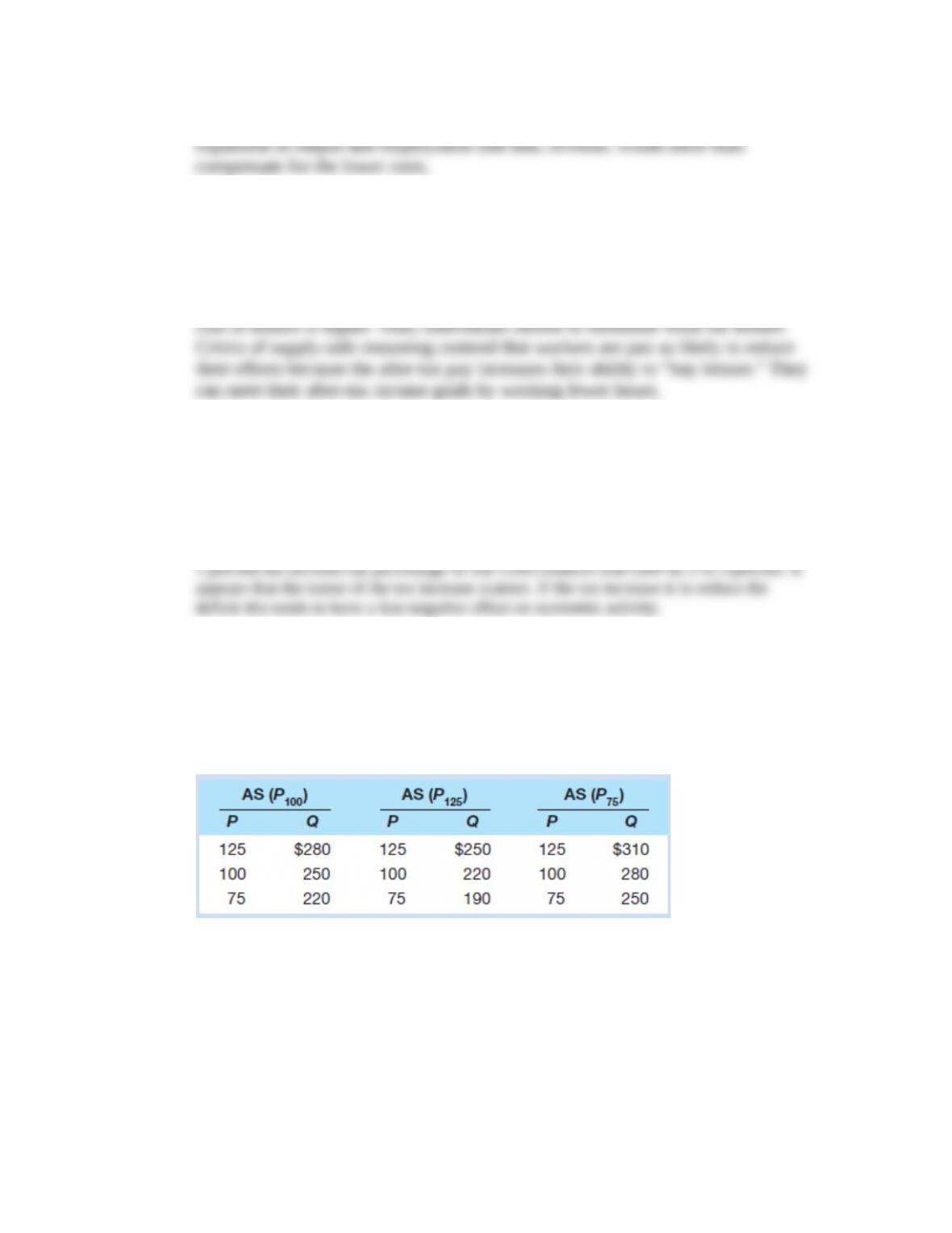
1. Suppose the full-employment level of real output (Q) for a hypothetical economy is $250 and
the price level (P) initially is 100. Use the short-run aggregate supply schedules below to answer
the questions that follow: LO1
a. What will be the level of real output in the short run if the price level unexpectedly rises from
100 to 125 because of an increase in aggregate demand? What if the price level unexpectedly falls
from 100 to 75 because of a decrease in aggregate demand? Explain each situation, using
numbers from the table.
b. What will be the level of real output in the long run when the price level rises from 100 to 125?
When it falls from 100 to 75? Explain each situation.
c. Show the circumstances described in parts a and b on graph paper, and derive the long-run
aggregate supply curve.
Answer:
18-3
Copyright © 2015 McGraw-Hill Education. All rights reserved. No reproduction or distribution without the prior written
consent of McGraw-Hill Education.
Chapter 18 – Extending the Analysis of Aggregate Supply
a. $280; $220. When the price level rises from 100 to 125 [in aggregate supply
Because nominal wages are constant, profits rise and producers increase output to
b. $250; $250. In the long run a rise in the price-level to 125 leads to nominal
c. Graphically, the explanation is identical to Figure 35.1b. Short-run AS: P1 =
2. Suppose that AD and AS intersect at an output level that is higher than the full-employment
output level. After the economy adjusts back to equilibrium in the long run, the price level will be
__________ . LO2
a. Higher than it is now.
b. Lower than it is now.
c. The same as it is now.
Feedback: After the economy adjusts back to equilibrium in the long run, the price level
will be higher than it is now. This is the case because when the economy is producing
output at a rate that is higher than the full-employment output level, there will be upward
3. Suppose that an economy begins in long-run equilibrium before the price level and real GDP
both decline simultaneously. If those changes were caused by only one curve shifting, then those
changes are best explained as the result of: LO2
a. The AD curve shifting right.
b. The AS curve shifting right.
c. The AD curve shifting left.
d. The AS curve shifting left.
18-4
Copyright © 2015 McGraw-Hill Education. All rights reserved. No reproduction or distribution without the prior written
consent of McGraw-Hill Education.
Chapter 18 – Extending the Analysis of Aggregate Supply
Feedback: If only one curve shifted, then this scenario in which the price level and real
GDP have recently declined can best be explained as the result of the AD curve shifting
By contrast, the incorrect answers all lead to outcomes that do not match the scenario that
4. Identify the two descriptions below as being the result of either cost-push inflation or demand-
pull inflation. LO2
a. Real GDP is below the full-employment level and prices have risen recently.
b. Real GDP is above the full-employment level and prices have risen recently.
Answer: a. Cost-push inflation: The situation in which “real GDP is below the full-
employment level and prices have risen recently” can be attributed to cost-push inflation
by noticing that if costs go up, the short-run aggregate supply curve will shift to the left.
b. Demand-pull inflation: By contrast, the situation in which “real GDP is above the full-
employment level and prices have risen recently” can be attributed to demand-pull
5. Use graphical analysis to show how each of the following would affect the economy first in the
short run and then in the long run. Assume that the United States is initially operating at its full-
employment level of output, that prices and wages are eventually flexible both upward and
downward, and that there is no counteracting fiscal or monetary policy. LO2
a. Because of a war abroad, the oil supply to the United States is disrupted, sending oil prices
rocketing upward.
b. Construction spending on new homes rises dramatically, greatly increasing total U.S.
investment spending.
c. Economic recession occurs abroad, significantly reducing foreign purchases of U.S. exports.
Answer:
a. See F igure 18.4 in the chapter, less AD2. Short run: The aggregate supply curve
18-5
Copyright © 2015 McGraw-Hill Education. All rights reserved. No reproduction or distribution without the prior written
consent of McGraw-Hill Education.
Chapter 18 – Extending the Analysis of Aggregate Supply
b. See F igure 18.3. Short run: The aggregate demand curve shifts to the right, and
c. See F igure 18.5. Short run: The aggregate demand curve shifts to the left, both
6. Between 1990 and 2009, the U.S. price level rose by about 64 percent while real output
increased by about 62 percent. Use the aggregate demand–aggregate supply model to illustrate
these outcomes graphically. LO2
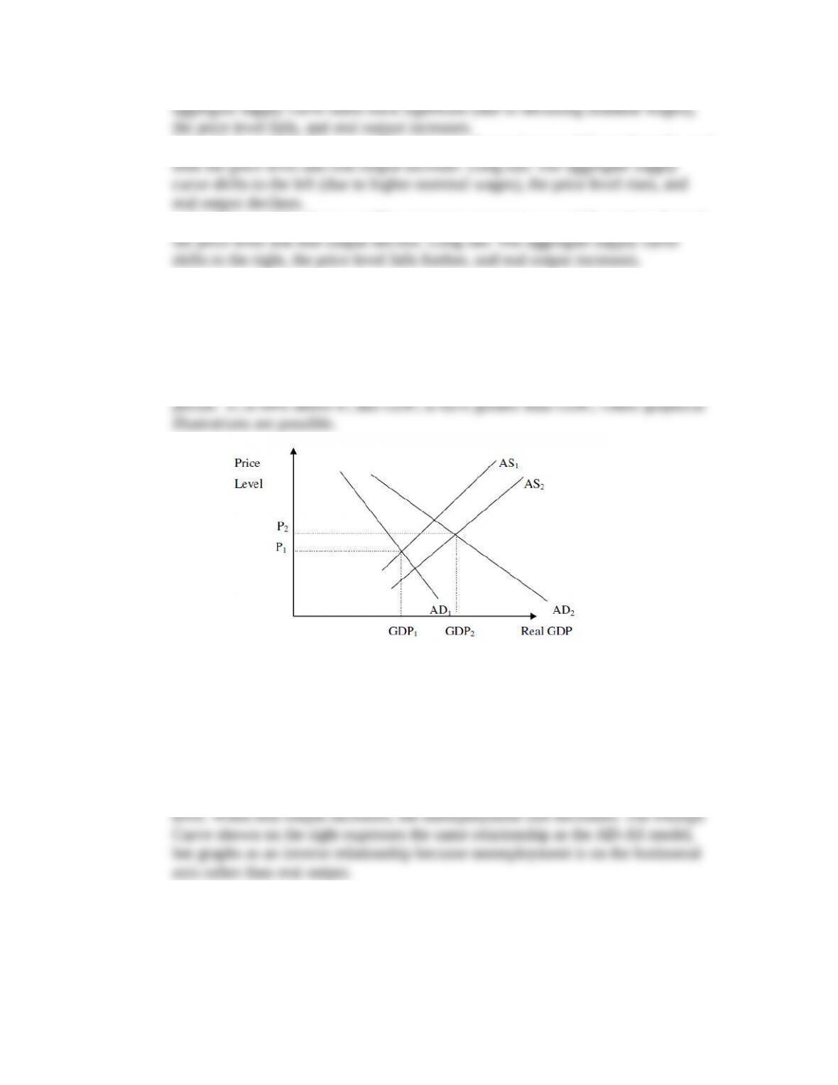
Answer: In the graph shown, both AD and AS expanded over the 1990-2009
7. Assume there is a particular short-run aggregate supply curve for an economy and the curve is
relevant for -several years. Use the AD-AS analysis to show graphically why higher rates of
inflation over this period would be associated with lower rates of unemployment, and vice versa.
What is this inverse relationship called? LO3
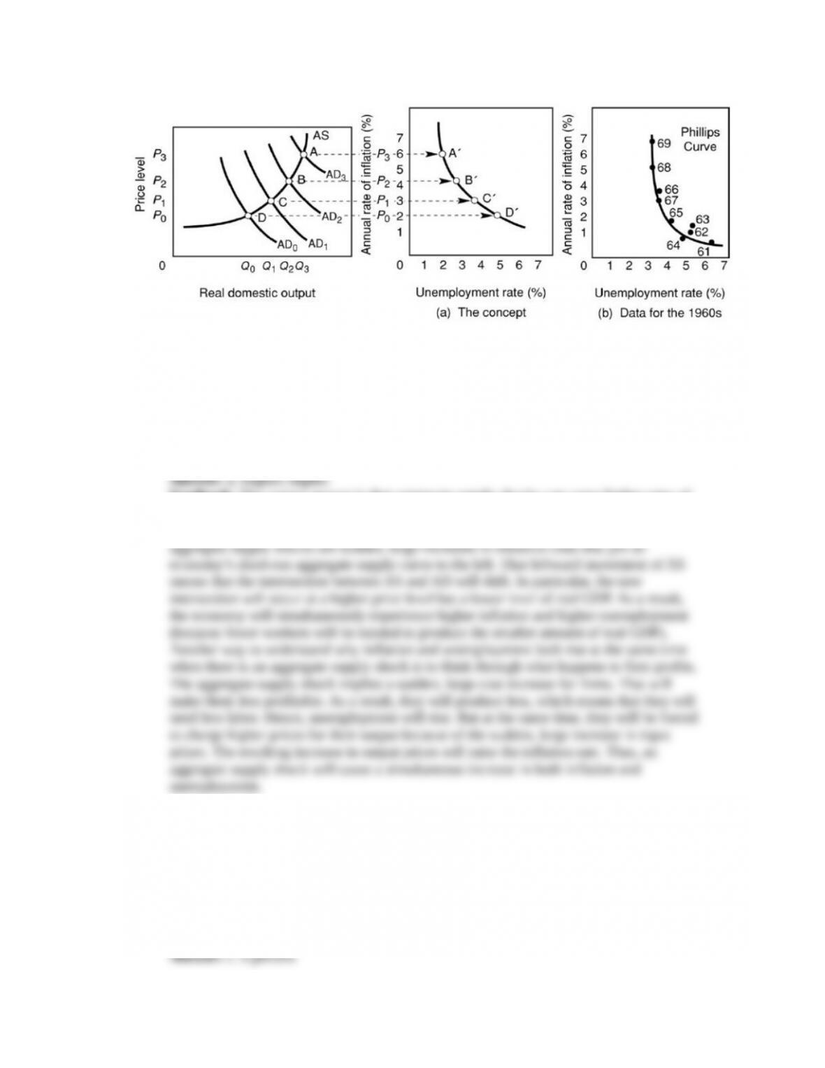
Answer: As aggregate demand increases given a particular short-run aggregate
supply curve, increases in real output are associated with increases in the price
18-6
Copyright © 2015 McGraw-Hill Education. All rights reserved. No reproduction or distribution without the prior written
consent of McGraw-Hill Education.
Chapter 18 – Extending the Analysis of Aggregate Supply
8. Aggregate supply shocks can cause ________ rates of inflation that are accompanied by
________ rates of unemployment. LO3
a. Higher; higher.
b. Higher; lower.
c. Lower; higher.
d. Lower; lower.
Feedback: The correct answer is that aggregate supply shocks can cause higher rates of
inflation that are accompanied by higher rates of unemployment.
This simultaneous increase in inflation and unemployment is driven by the fact that
9. Suppose that firms are expecting 6 percent inflation while workers are expecting 9 percent
inflation. How much of a pay raise will workers demand if their goal is to maintain the
purchasing power of their incomes? LO4
a. 3 percent.
b. 6 percent.
c. 9 percent.
d. 12 percent.
18-7
Copyright © 2015 McGraw-Hill Education. All rights reserved. No reproduction or distribution without the prior written
consent of McGraw-Hill Education.
Chapter 18 – Extending the Analysis of Aggregate Supply
Feedback: Workers will demand a 9 percent pay raise if their goal is to maintain the
purchasing power of their incomes.
In general, workers’ salary demands will mirror the inflation rate that they are expecting.
10. Suppose that firms were expecting inflation to be 3 percent, but then it actually turned out to
be 7 percent. Other things equal, firm profits will be: LO4
a. Smaller than expected.
b. Larger than expected.
Feedback: The correct answer is that if the firm‘s input suppliers act on their expectation
of 3 percent inflation, the firm’s profits will turn out to larger than expected.
PROBLEMS
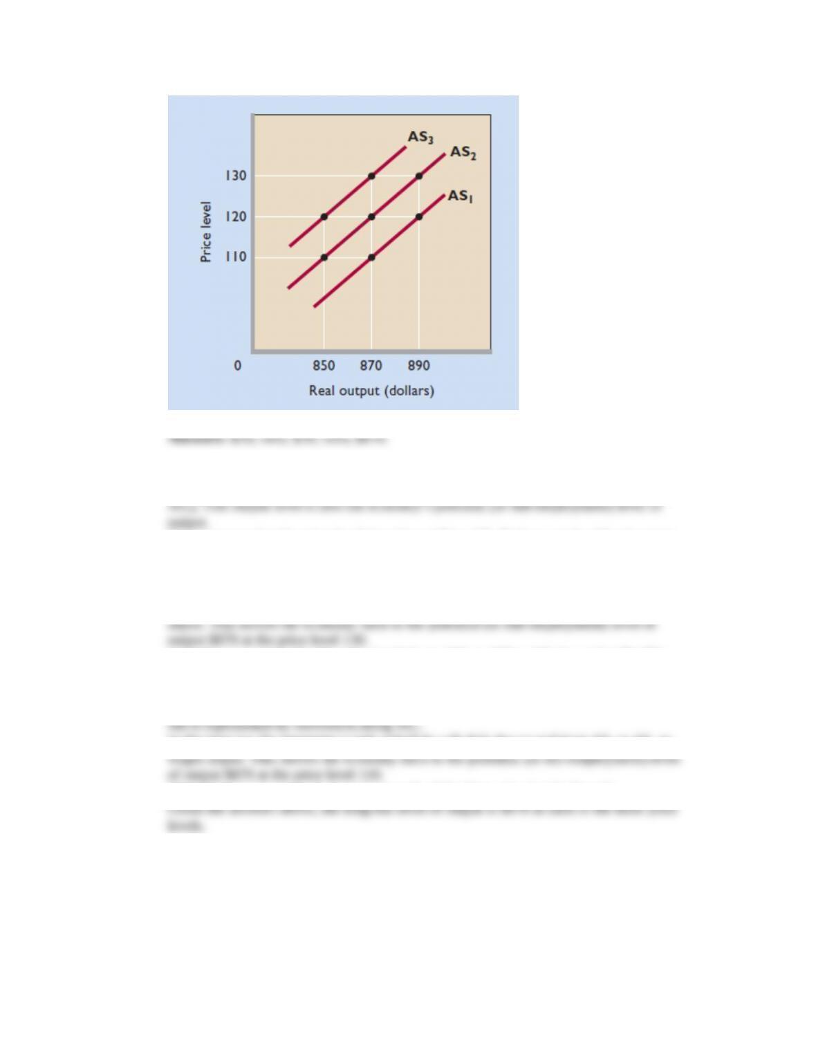
1. Use the accompanying figure to answer the follow questions. Assume that the economy
initially is operating at price level 120 and real output level $870. This output level is the
economy’s potential (or full-employment) level of output. Next, suppose that the price level rises
from 120 to 130. By how much will real output increase in the short run? In the long-run?
Instead, now assume that the price level dropped from 120 to 110. Assuming flexible product and
resource prices, by how much will real output fall in the short run? In the long run? What is the
long-run level of output at each of the three price levels shown? LO1
18-8
Copyright © 2015 McGraw-Hill Education. All rights reserved. No reproduction or distribution without the prior written
consent of McGraw-Hill Education.
Chapter 18 – Extending the Analysis of Aggregate Supply
Feedback:
The economy is initially operating at the price level 120 and real output level $870 (on
Next, suppose that the price level rises from 120 to 130. By how much will real output
increase in the short run? In the long-run?
In the short run aggregate supply will increase to $890, which is an increase of $20. The
short run is represented by movement along AS2.
In the long run the aggregate supply schedule will shift upward from AS2 to AS3 as wages
Instead, now assume that the price level dropped from 120 to 110. Assuming flexible
product and resource prices, by how much will real output fall in the short run? In the
long run?
In the short run aggregate supply will fall to $850, which is a decrease of $20. The short
In the long run the aggregate supply schedule will shift downward from AS2 to AS1 as
What is the long-run level of output at each of the three price levels shown?
2. ADVANCED ANALYSIS Suppose that the equation for a particular short-run AS curve is P =
20 + .5Q, where P is the price level and Q is real output in dollar terms. What is Q if the price
level is 120? Suppose that the Q in your answer is the full-employment level of output. By how
much will Q increase in the short run if the price level unexpectedly rises from 120 to 132? By
how much will Q increase in the long-run due to the price level increase? LO1
18-9
Copyright © 2015 McGraw-Hill Education. All rights reserved. No reproduction or distribution without the prior written
consent of McGraw-Hill Education.
Chapter 18 – Extending the Analysis of Aggregate Supply
Feedback:
Since we are given the price level we need to solve the short-run AS curve for Q as a
function of P.
What is Q if the price level is 120?
Assume this answer is the full-employment level of output.
By how much will Q increase in the short run if the price level unexpectedly rises from
120 to 132?
The change in Q is 24.
By how much will Q increase in the long-run due to the price level increase?
3. Suppose that over a 30-year period Buskerville’s price level increased from 72 to 138 while its
real GDP rose from $1.2 trillion to $2.1 trillion. Did economic growth occur in Buskerville? If so,
by what average yearly rate? Did Buskerville experience inflation? If so, by what average yearly
rate? Which shifted rightward faster in Buskerville: its long-run aggregate supply curve (ASLR)
or its aggregate demand curve (AD)? LO2
Feedback: Yes, real GDO rose over this time period.
If so, by what average yearly rate?
First, find the rate of growth for the given period of time (30 year period in this example).
To find the average annual rate of growth divide by the number of years in the period.
Did Buskerville experience inflation?
Yes, the price level rose over this period.
If so, by what average yearly rate?
First, find the inflation rate for the given period of time (30 year period in this example).
To find the average inflation rate divide by the number of years in the period.
Which shifted rightward faster in Buskerville: its long-run aggregate supply curve
(ASLR) or its aggregate demand curve (AD)?
The AD schedule because the price level increased over this period of time.
4. Suppose that for years East Confetti’s short-run Phillips Curve was such that each 1 percentage
point increase in its unemployment rate was associated with a 2 percentage point decline in its
inflation rate. Then, during several recent years the short run pattern changed such that its
inflation rate rose by 3 percentage points for every 1 percentage point drop in its unemployment
rate. Graphically, did East Confetti’s Phillips Curve shift upward or did it shift downward? LO3
18-10
Copyright © 2015 McGraw-Hill Education. All rights reserved. No reproduction or distribution without the prior written
consent of McGraw-Hill Education.
Chapter 18 – Extending the Analysis of Aggregate Supply
Feedback:
The answer is upward.
The logic is as follows. The trade-off between inflation and unemployment is 2
18-11
Copyright © 2015 McGraw-Hill Education. All rights reserved. No reproduction or distribution without the prior written
consent of McGraw-Hill Education.