Chapter 11 – The Aggregate Expenditures Model
PROBLEMS
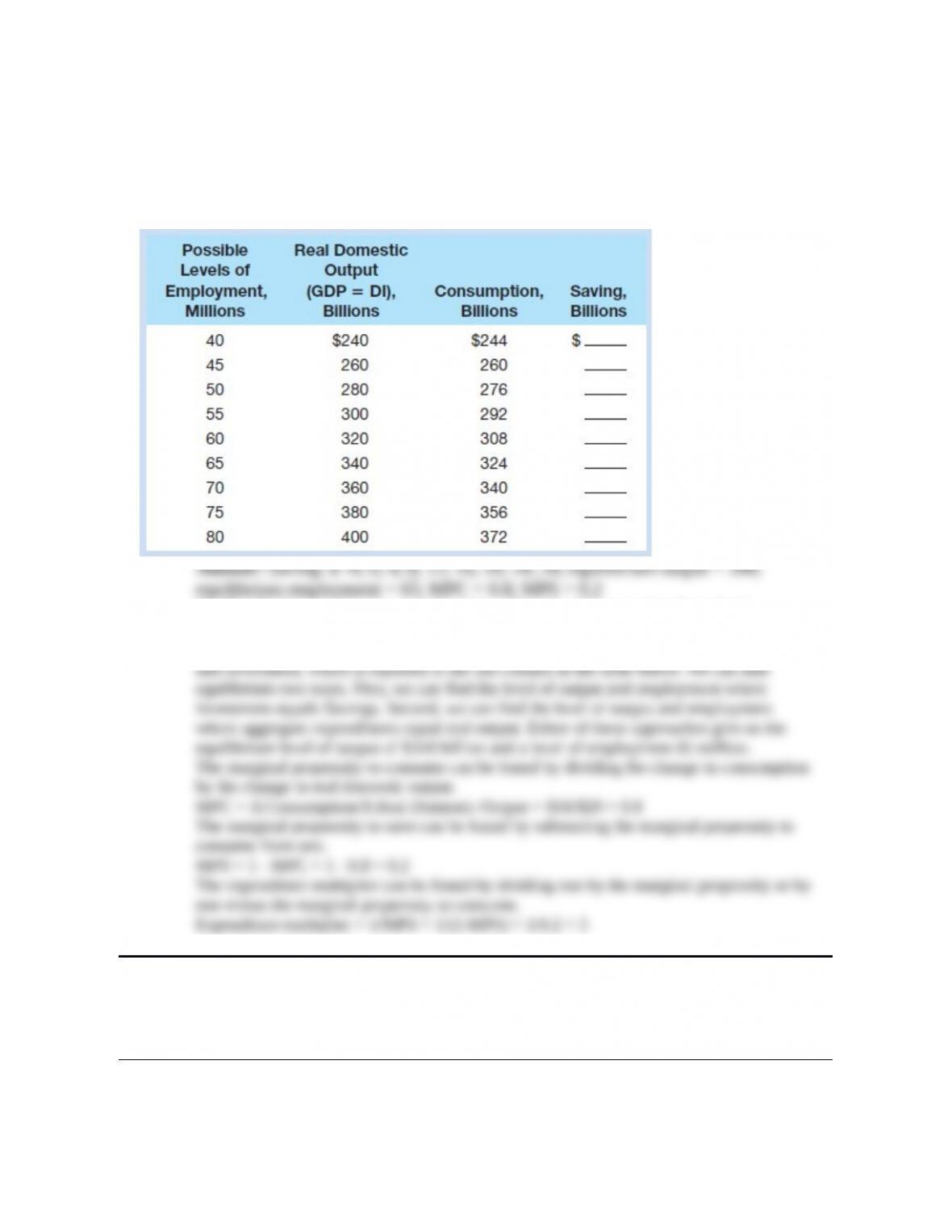
1. Assuming the level of investment is $16 billion and independent of the level of total output,
complete the accompanying table and determine the equilibrium levels of output and employment
in this private closed economy. What are the sizes of the MPC and MPS? LO3
Feedback: The savings column is found by subtracting Consumption from Real
Domestic Output (disposable income) for each row. The answers are reported in the
savings column below. We can also find aggregate expenditures by adding consumption
Possible levels
of
employment
(millions)
Real domestic
output
(GDP=DI)
(billions)
Consumption
(billions)
Saving
(billions
)
Investment
(billions)
Aggregate
Expenditures
(billions)
11-1
Copyright © 2015 McGraw-Hill Education. All rights reserved. No reproduction or distribution without the prior written
consent of McGraw-Hill Education.
Chapter 11 – The Aggregate Expenditures Model
40
$240
$244
$ -4
$16
$260
2. Using the consumption and saving data in problem 1 and assuming investment is $16 billion,
what are saving and planned investment at the $380 billion level of domestic output? What are
saving and actual investment at that level? What are saving and planned investment at the $300
billion level of domestic output? What are the levels of saving and actual investment? In which
direction and by what amount will unplanned investment change as the economy moves from the
$380 billion level of GDP to the equilibrium level of real GDP? From the $300 billion level of
real GDP to the equilibrium level of GDP? LO4
Answer: At $380 billion level, saving = $24 billion; planned investment = $16
billion. Actual saving = $24 billion; actual investment is $24 billion
Feedback: At the $380 billion level of GDP, saving = $24 billion; planned investment =
$16 billion (from the question). This deficiency of $8 billion of planned investment
At the $300 billion level of GDP, saving = $8 billion; planned investment = $16
billion (from the question). This excess of $8 billion of planned investment
When unplanned investments in inventories occur, as at the $380 billion level of
GDP, businesses revise their production plans downward and GDP falls. When
3. By how much will GDP change if firms increase their investment by $8 billion and the MPC
is .80? If the MPC is .67? LO5
11-2
Copyright © 2015 McGraw-Hill Education. All rights reserved. No reproduction or distribution without the prior written
consent of McGraw-Hill Education.
Chapter 11 – The Aggregate Expenditures Model
Feedback: First, we need to find the expenditure multiplier. The expenditure multiplier
can be found by dividing one by one minus the marginal propensity to consume.
Expenditure multiplier = 1/(1-MPC)
4. Suppose that a certain country has an MPC of .9 and a real GDP of $400 billion. If its
investment spending decreases by $4 billion, what will be its new level of real GDP? LO5
Feedback: First, we need to find the expenditure multiplier. The expenditure multiplier
can be found by dividing one by one minus the marginal propensity to consume.
For our value, we have an expenditure multiplier of 10 (= 1/(1-0.9)).
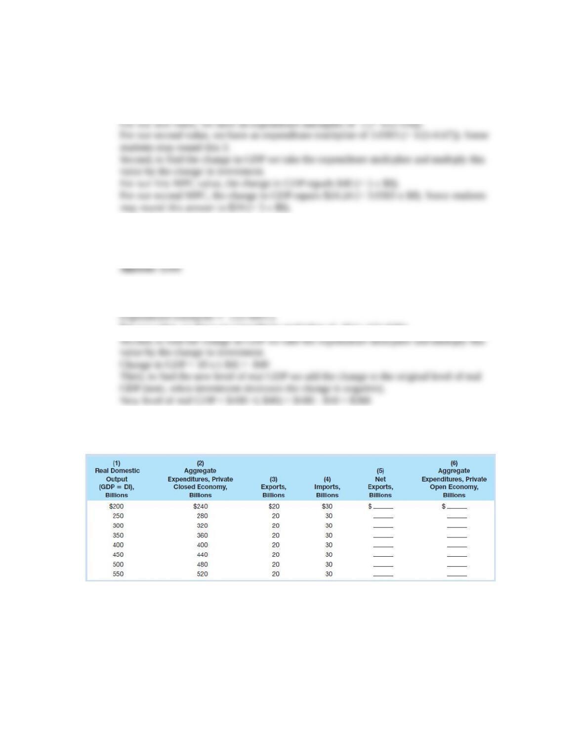
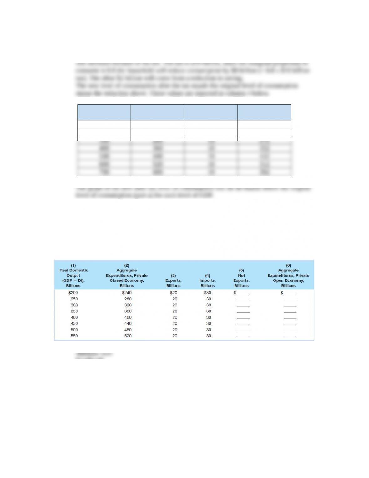
5. The data in columns 1 and 2 in the accompanying table are for a private closed economy: LO6
a. Use columns 1 and 2 to determine the equilibrium GDP for this hypothetical economy.
b. Now open up this economy to international trade by including the export and import
figures of columns 3 and 4. Fill in columns 5 and 6 and determine the equilibrium GDP
for the open economy. What is the change in equilibrium GDP caused by the addition of
net exports?
c. Given the original $20 billion level of exports, what would be net exports and the
equilibrium GDP if imports were $10 billion greater at each level of GDP?
11-3
Copyright © 2015 McGraw-Hill Education. All rights reserved. No reproduction or distribution without the prior written
consent of McGraw-Hill Education.
Chapter 11 – The Aggregate Expenditures Model
d. What is the multiplier in this example?
b. Column 5: -$ 10; -$ 10; -$ 10; -$ 10; -$ 10; -$ 10; -$ 10; -$ 10; Column 6: $
d. 5
Feedback: Part a:
a. Equilibrium for this economy occurs where Aggregate Expenditures for the Private
(1)
Real
domestic
output
(GDP=DI)
billions
(2)
Aggregate
Expenditures,
private closed
economy,
billions
(3)
Exports,
billions
(4)
Imports,
billions
(5)
Net
exports,
private
economy
(6)
Aggregate
expenditures,
open
billions
$200
$250
$240
$280
$20
$20
$30
$30
-$ 10
-$ 10
$ 230
$ 270
Equilibrium for this economy occurs where Aggregate Expenditures for the Private Open
11-4
Copyright © 2015 McGraw-Hill Education. All rights reserved. No reproduction or distribution without the prior written
consent of McGraw-Hill Education.
Chapter 11 – The Aggregate Expenditures Model
(1)
Real
domestic
output
(GDP=DI)
billions
(2)
Aggregate
Expenditures,
private closed
economy,
billions
(3)
Exports,
billions
(4)
Imports,
billions
(5)
Net
exports,
private
economy
(6)
Aggregate
expenditures,
open
billions
$200
$240
$20
$40
-$ 20
$ 220
Equilibrium for this economy occurs where Aggregate Expenditures for the Private Open
Part d:
To find the multiplier for this example we could use the standard approach using the
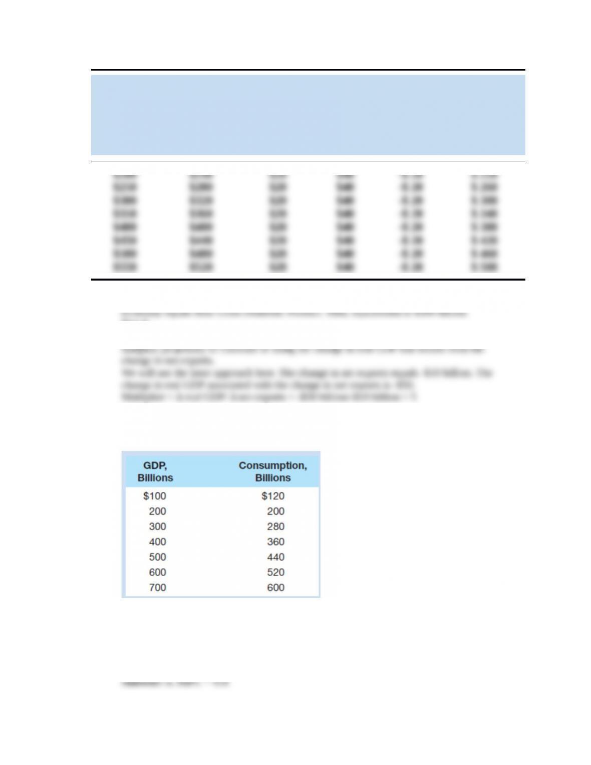
6. Assume that, without taxes, the consumption schedule of an economy is as follows: LO7
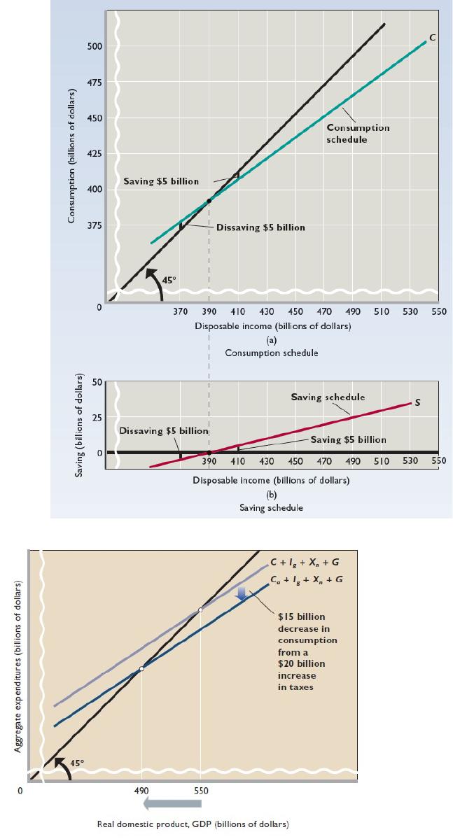
a. Graph this consumption schedule and determine the MPC.
b. Assume now that a lump-sum tax is imposed such that the government collects $10
billion in taxes at all levels of GDP. Graph the resulting consumption schedule and
compare the MPC and the multiplier with those of the pretax consumption schedule.
11-5
Copyright © 2015 McGraw-Hill Education. All rights reserved. No reproduction or distribution without the prior written
consent of McGraw-Hill Education.
Chapter 11 – The Aggregate Expenditures Model
b. Multiplier before tax = 5
Refer to below figures for the graphs for (a) and (b) respectively.
11-6
Copyright © 2015 McGraw-Hill Education. All rights reserved. No reproduction or distribution without the prior written
consent of McGraw-Hill Education.
Chapter 11 – The Aggregate Expenditures Model
Part a:
Use the values in the table above for graph. The size of the MPC is 80/100 or .8
because consumption changes by 80 when GDP changes by 100.
11-7
Copyright © 2015 McGraw-Hill Education. All rights reserved. No reproduction or distribution without the prior written
consent of McGraw-Hill Education.
Chapter 11 – The Aggregate Expenditures Model
Part b:
To find the level of consumption after the tax we first find out by how much consumption
GDP, Billions Consumption
before Tax
Tax Consumption
after Tax
$100 $120 $10 $112
200 200 10 192
7. Refer to columns 1 and 6 in the table for problem 5. Incorporate government into the table by
assuming that it plans to tax and spend $20 billion at each possible level of GDP. Also assume
that the tax is a personal tax and that government spending does not induce a shift in the private
aggregate expenditures schedule. What is the change in equilibrium GDP caused by the addition
of government? LO7
Feedback:
11-8
Copyright © 2015 McGraw-Hill Education. All rights reserved. No reproduction or distribution without the prior written
consent of McGraw-Hill Education.
Chapter 11 – The Aggregate Expenditures Model
(1)
Real
domestic
output
(GDP=DI)
billions
(2)
Aggregate
Expenditures,
private closed
economy,
billions
(3)
Exports,
billions
(4)
Imports,
billions
(5)
Net
exports,
private
economy
(6)
Aggregate
expenditures,
open
billions
$200
$250
$240
$280
$20
$20
$30
$30
-$ 10
-$ 10
$ 230
$ 270
(NOTE: Use marginal propensity to consume and multiplier found in problem 5)
Before G is added, open private sector equilibrium will be at $350. The addition
The addition of government expenditures G to our analysis raises the aggregate
expenditures (C + Ig +Xn + G) schedule and increases the equilibrium level of
GDP. This change in government spending is subject to the multiplier effect.
The $20 billion increase in T reduces initially reduces consumption by $16 billion
8. ADVANCED ANALYSIS Assume that the consumption schedule for a private open economy
is such that consumption C = 50 + 0.8Y. Assume further that planned investment Ig and net
exports Xn are independent of the level of real GDP and constant at Ig = 30 and Xn = 10. Recall
also that, in equilibrium, the real output produced (Y) is equal to aggregate expenditures: Y = C +
Ig + Xn. LO7
a. Calculate the equilibrium level of income or real GDP for this economy.
b. What happens to equilibrium Y if Ig changes to 10? What does this outcome reveal about the
size of the multiplier?
Part b:
If Investment falls from 30 to 10, we follow the same procedure (except let Ig=10).
In equilibrium we have the following relationship:
The multiplier can be found by dividing the change in output (Y) by the change in
investment (Ig).
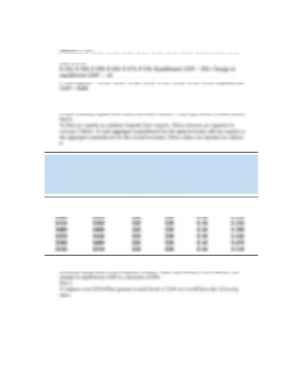
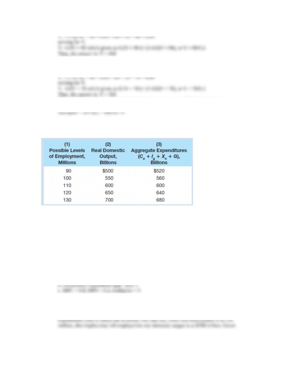
9. Refer to the accompanying table in answering the questions that follow: LO8
a. If full employment in this economy is 130 million, will there be an inflationary expenditure gap
or a recessionary expenditure gap? What will be the consequence of this gap? By how much
would aggregate expenditures in column 3 have to change at each level of GDP to eliminate the
inflationary expenditure gap or the recessionary expenditure gap? What is the multiplier in this
example?
b. Will there be an inflationary expenditure gap or a recessionary expenditure gap if the full-
employment level of output is $500 billion? By how much would aggregate expenditures in
column 3 have to change at each level of GDP to eliminate the gap? What is the multiplier in this
example?
c. Assuming that investment, net exports, and government expenditures do not change with
changes in real GDP, what are the sizes of the MPC, the MPS, and the multiplier?
Answer: a. Recessionary expenditure gap; 20 billion shortfall of employment; $20; 5
Feedback:
Part a:
The equilibrium in this economy is at $600 billion, real domestic output equals aggregate
11-10
Copyright © 2015 McGraw-Hill Education. All rights reserved. No reproduction or distribution without the prior written
consent of McGraw-Hill Education.
Chapter 11 – The Aggregate Expenditures Model
If aggregate expenditures increased by $20 billion the new equilibrium would be at $700
billion, which is at full employment (add $20 billion to each level of aggregate
Part b:
Again, the equilibrium in this economy is at $600 billion, real domestic output equals
aggregate expenditures (this is where the economy will take us). Since full employment
If aggregate expenditures decreased by $20 billion, for this case, the new equilibrium
would be at $500 billion, which is at full employment (subtract $20 billion from each
(note the changes are negative in this case)
Part c:
To find the marginal propensity to consume (MPC) divide the change in aggregate
expenditures by the change in real domestic output (assuming that investment, net
10. Answer the following questions, which relate to the aggregate expenditures model: LO8
a. If C is $100, Ig is $50, Xn is –$10, and G is $30, what is the economy’s equilibrium GDP?
b. If real GDP in an economy is currently $200, C is $100, Ig is $50, Xn is -$10, and G is $30,
will the economy’s real GDP rise, fall, or stay the same?
c. Suppose that full-employment (and full-capacity) output in an economy is $200. If C is $150,
Ig is $50, Xn is –$10, and G is $30, what will be the macroeconomic result?
Answer: a. $170
Feedback:
Part a:
Equilibrium occurs where real output (Y) equals aggregate expenditures (AE), where AE
= C + Ig + G +Xn.
Using this relationship, we have the equilibrium value:
11-11
Copyright © 2015 McGraw-Hill Education. All rights reserved. No reproduction or distribution without the prior written
consent of McGraw-Hill Education.
Chapter 11 – The Aggregate Expenditures Model
Part b:
If real GDP is $200, aggregate expenditures of $170 will result in positive
Part c:
Here we can use the same approach as in part (a)
11-12
Copyright © 2015 McGraw-Hill Education. All rights reserved. No reproduction or distribution without the prior written
consent of McGraw-Hill Education.