Unlock document.
This document is partially blurred.
Unlock all pages and 1 million more documents.
Get Access
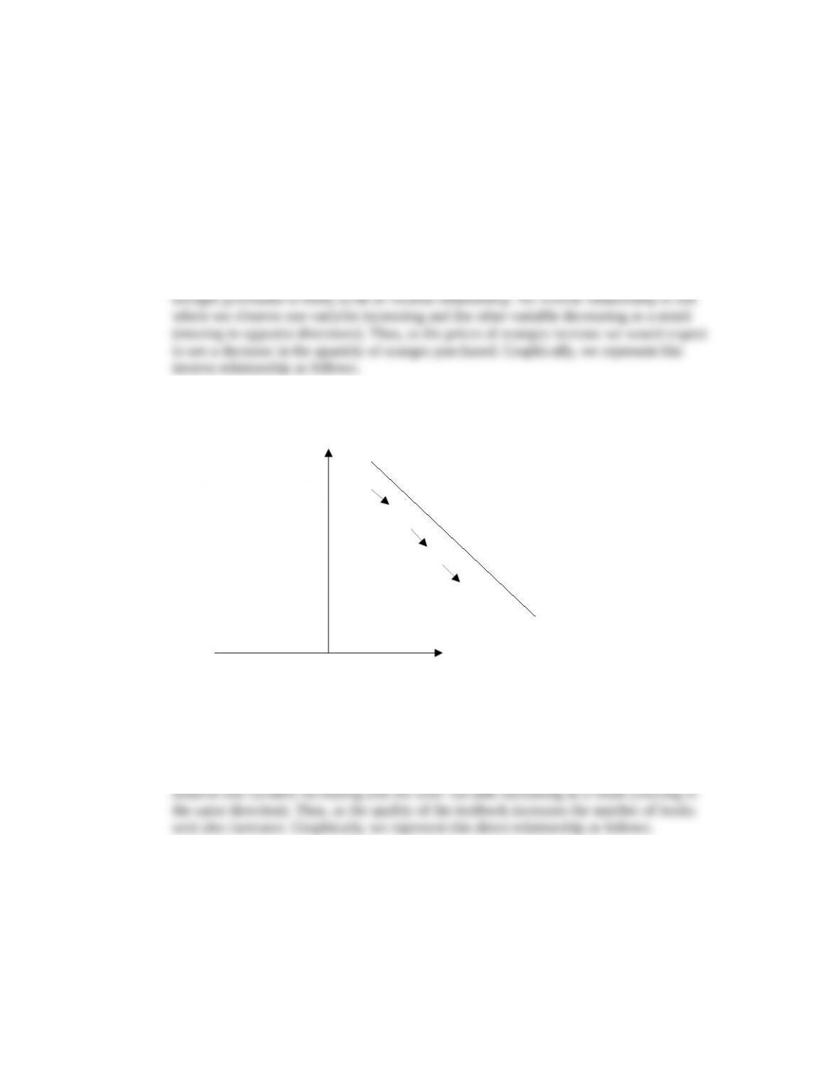
Price of Oranges
Quantity of Oranges
Inverse Relationship
Chapter 01 Appendix
Chapter 01 Appendix
McConnell Brue Flynn 20e
APPENDIX DISCUSSION QUESTIONS
1. Briefly explain the use of graphs as a way to represent economic relationships. What is an
inverse relationship? How does it graph? What is a direct relationship? How does it graph? LO8
Answer: Graphs help us visualize relationships between key economic variables in the
data. For example, the relationship between the price of oranges and the number of
As another example, the relationship between the quality of a textbook and the number of
textbooks sold is likely to be a direct relationship. A direct relationship is one where we
1A-1
Copyright © 2015 McGraw-Hill Education. All rights reserved. No reproduction or distribution without the prior written
consent of McGraw-Hill Education.

Number of Textbooks Sold
Quality of the Textbook
Direct Relationship
Chapter 01 Appendix
2. Describe the graphical relationship between ticket prices and the number of people choosing to
visit amusement parks. Is that relationship consistent with the fact that, historically, park
attendance and ticket prices have both risen? Explain. LO8
Answer: There is likely an inverse relationship between ticket prices and the number of
The fact that, historically, park attendance and ticket prices have both risen over time
3. Look back at Figure 2, which shows the inverse relationship between ticket prices and game
attendance at Gigantic State University. (a) Interpret the meaning of both the slope and the
intercept. (b) If the slope of the line were steeper, what would that say about the amount by which
ticket sales respond to increases in ticket prices? (c) If the slope of the line stayed the same but
the intercept increased, what can you say about the amount by which ticket sales respond to
increases in ticket prices? LO8
1A-2
Copyright © 2015 McGraw-Hill Education. All rights reserved. No reproduction or distribution without the prior written
consent of McGraw-Hill Education.
Chapter 01 Appendix
Answer:
Part a: The slope of this relationship tells us how much the price of a ticket must fall to
induce someone to buy an additional ticket. In this case, the slope of -2.5 tells us that the
Part b: If the slope of this line were steeper this would imply that the price must fall by
Part c: If the vertical intercept increased this would imply that individuals are willing to
APPENDIX REVIEW QUESTIONS
1. Indicate whether each of the following relationships is usually a direct relationship or
an inverse relationship. LO8
a. A sports team's winning percentage and attendance at its home games.
b. Higher temperature and sweater sales.
c. A person's income and how often they shop at discount stores.
d. Higher gasoline prices and miles driven in automobiles.
Answer:
Part a: direct relationship because winning reams are typically more popular.
Part b: inverse relationship because as higher temperatures people usually
purchase fewer sweaters
2. Erin grows pecans. The number of bushels (B) that she can produce depends on the
number of inches of rainfall (R) that her orchards get. The relationship is given
algebraically as follows: B = 3,000 + 800R. Match each part of this equation with the
correct term. LO8
Bslope
3,000 dependent variable
800 vertical intercept
Rindependent variable
1A-3
Copyright © 2015 McGraw-Hill Education. All rights reserved. No reproduction or distribution without the prior written
consent of McGraw-Hill Education.

Sale of Umbrellas
Inches of Rainfall
Direct Relationship
Chapter 01 Appendix
Answer:
B goes with dependent variable.
APPENDIX PROBLEMS
1. Graph and label as either direct or indirect the relationships you would expect to find between
(a) the number of inches of rainfall per month and the sale of umbrellas, (b) the amount of tuition
and the level of enrollment at a university, and (c) the popularity of an entertainer and the price of
her concert tickets. LO8
Answer:
Part a:
Part b:
1A-4
Copyright © 2015 McGraw-Hill Education. All rights reserved. No reproduction or distribution without the prior written
consent of McGraw-Hill Education.
Student Enrollment
Tuition
Inverse Relationship
Price of Concert Tickets
Popularity of the Entertainer
Direct Relationship
Chapter 01 Appendix
Part c:
Feedback: Consider the following situations:
Part a: The number of inches of rainfall per month and the sale of umbrellas: There is
likely a direct relationship between the number of inches of rainfall per month and the
sale of umbrellas (more rain implies more umbrellas).
1A-5
Copyright © 2015 McGraw-Hill Education. All rights reserved. No reproduction or distribution without the prior written
consent of McGraw-Hill Education.
Sale of Umbrellas
Inches of Rainfall
Direct Relationship
Student Enrollment
Tuition
Inverse Relationship
Chapter 01 Appendix
Part b: The amount of tuition and the level of enrollment at a university: There is likely
an inverse relationship between the amount of tuition and the level of enrollment at a
university. As tuition increases less students will attend the university.
1A-6
Copyright © 2015 McGraw-Hill Education. All rights reserved. No reproduction or distribution without the prior written
consent of McGraw-Hill Education.

Price of Concert Tickets
Popularity of the Entertainer
Direct Relationship
Chapter 01 Appendix
Part c: The popularity of an entertainer and the price of her concert tickets: There is likely
a direct relationship between the popularity of an entertainer and the price of her concert
tickets. The more popular the entertainer, the more people are willing to pay to see her in
concert.
2. Indicate how each of the following might affect the data shown in the table and graph in
Figure 2 of this appendix: LO8
a. GSU’s athletic director schedules higher-quality opponents.
b. An NBA team locates in the city where GSU plays.
c. GSU contracts to have all its home games televised.
Feedback: Consider the three scenarios:
Part a: GSU’s athletic director schedules higher-quality opponents. By scheduling higher
Part b: An NBA team locates in the city where GSU plays. If an NBA team locates in the
Part c: GSU contracts to have all its home games televised. If GSU contracts to have all
1A-7
Copyright © 2015 McGraw-Hill Education. All rights reserved. No reproduction or distribution without the prior written
consent of McGraw-Hill Education.
Chapter 01 Appendix
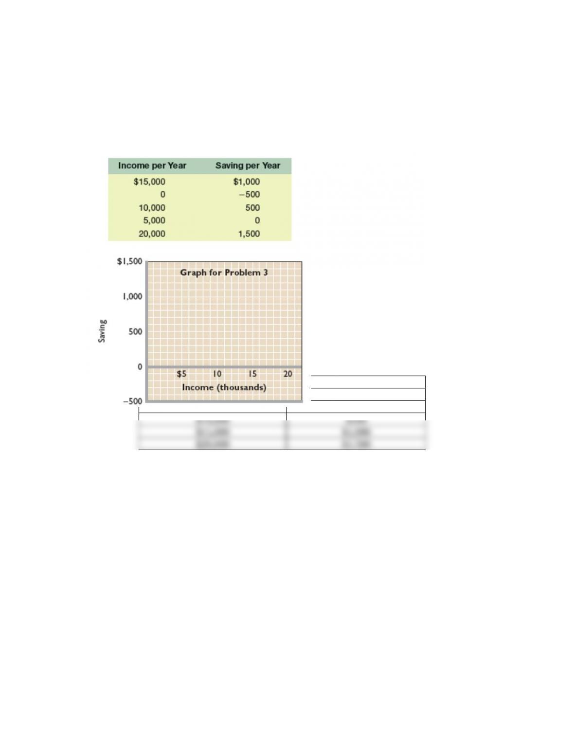
3. The following table contains data on the relationship between saving and income. Rearrange
these data into a logical order and graph them on the accompanying grid. What is the slope of the
line? The vertical intercept? Write the equation that represents this line. What would you predict
saving to be at the $12,500 level of income? LO8
Answer:
Income per Year Saving per Year
0 -$500
$5,000 0
1A-8
Copyright © 2015 McGraw-Hill Education. All rights reserved. No reproduction or distribution without the prior written
consent of McGraw-Hill Education.

Chapter 01 Appendix
Saving per Year
Slope equals (500/5000) or 0.10; the vertical intercept equals -$500. The equation
Feedback: Consider the following data:
Income per Year Saving per Year
$15,000 $1,000
0 -$500
To rearrange the above data into a meaningful order, we start with the lowest income and
saving pair. We then continue with sequentially higher values of both income and saving.
Income per Year Saving per Year
0 -$500
$5,000 0
Graphically, we have the following.
1A-9
Copyright © 2015 McGraw-Hill Education. All rights reserved. No reproduction or distribution without the prior written
consent of McGraw-Hill Education.

Chapter 01 Appendix
Saving per Year
The slope of the saving line can be found by dividing the change in saving by the change
in income between any two points. For example we have the entry (5000 (income), 0
(savings)) and the entry (10000 (income), 500 (savings)). This implies that the change in
To find the predicted amount of saving for a given level of income we substitute the
1A-10
Copyright © 2015 McGraw-Hill Education. All rights reserved. No reproduction or distribution without the prior written
consent of McGraw-Hill Education.


