Chapter 06 – Efficient Diversification
CHAPTER SIX
EFFICIENT DIVERSIFICATION
CHAPTER OVERVIEW
In this chapter, the concept of portfolio formation moves beyond the risky and risk-free asset
that is tangent to the so called efficient frontier of best diversified portfolios, will dominate all
risky portfolios regardless of the level of risk aversion.
As in Chapter 5, investors will optimally vary their asset-allocation decision according to their risk
tolerance by varying the amount they invest in the tangency portfolio and the amount invested in
the risk free asset. See Text figure 6.6. The single-factor-index model is introduced; which
find the minimum variance combinations of two securities. Upon completion of this chapter the
student should have a full understanding of systematic and firm-specific risk, and of how the
portfolio’s firm-specific risk can be reduced by combining securities with differing patterns of
returns. The student should be able to quantify this concept by being able to calculate and
interpret covariance and correlation coefficients.
and thus determine the firm‘s reaction to macroeconomic (market) events.
In addition, the students should be able to construct portfolios of different risk levels, given
information about risk-free rates and returns on risky assets or portfolios of risky assets. Students
should be able to calculate the expected return and standard deviation of these portfolios.
CHAPTER OUTLINE
1. Diversification and Portfolio Risk
2. Asset Allocation with Two Risky Assets
PPT 6-2 through PPT 6-17
When we put stocks in a portfolio, sp < S(Wisi). When Stock 1 has a return > E[r1], it is likely
that Stock 2 has a return < E[r2] so that return on the portfolio that contains stocks 1 and 2
remains close to its expected return. Covariance and correlation measure the tendency for r1 to
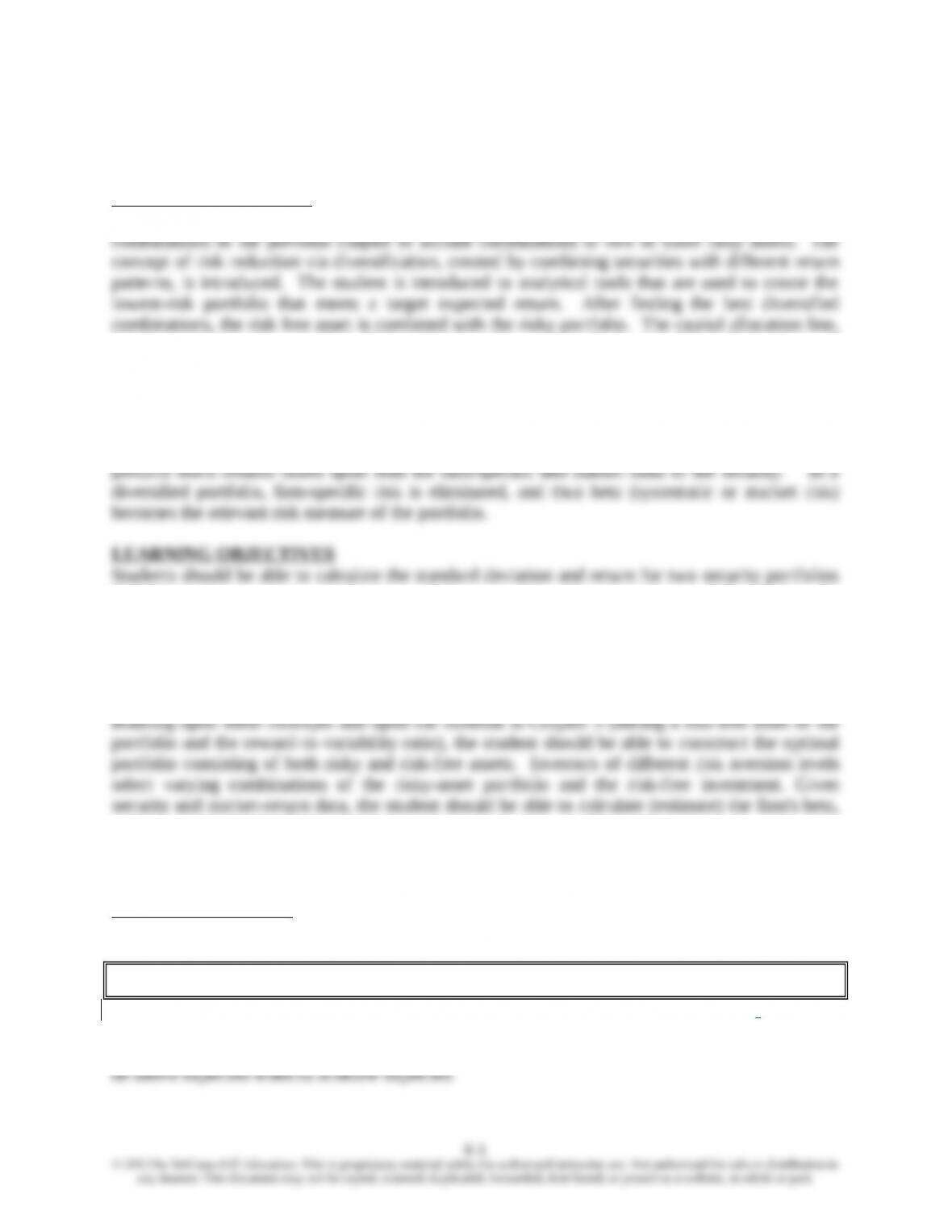
Text Figure 6.2 illustrates how adding securities to the portfolio reduces the portfolio risk as
measured by the standard deviation. Notice size of the standard deviation of a single stock
portfolio. At about 50%, holding a single stock is extremely risky. If the stock has an expected
return of 15% and a standard deviation of 50% then the investor can expect a very wide range of
possible returns of +65% and -35% two out of three years. These stocks were randomly selected
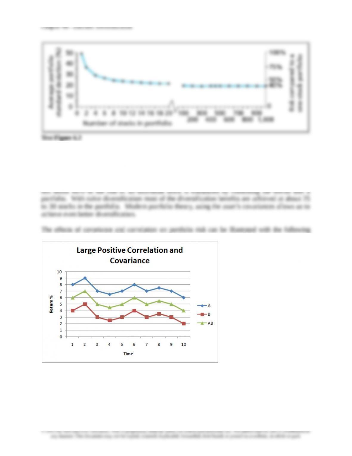
graphs that are also in the PPT:
Assets A and B have positive standard deviations and the correlation between A and B is +1.
Thus, the standard deviation of Portfolio AB is a simple weighted average of the standard
deviations of A and B and no risk is reduced by combining the two.
6-2
averaged or diversified away.
Return and Risk of a Two Asset Portfolio
The expected return of a portfolio is simply a weighted average of the returns of the portfolio
components. Because of the diversification effects however, the standard deviation of the
portfolio is not a simple weighted average of standard deviations of the components. The relevant
Cov(r1r2) = Covariance of returns for Security 1 and Security 2
6-3
Chapter 06 – Efficient Diversification
The PPT provides ample detail about the correlation coefficient and about why correlations are
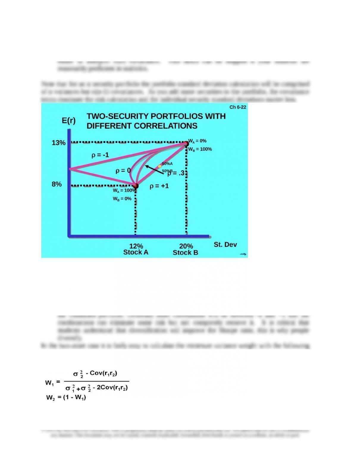
The graph depicts return/risk combinations of two securities, A and B for different hypothetical
correlation coefficients. If there is a perfect positive correlation between A and B,
combining the two securities yields no diversification benefits and combinations of A and B
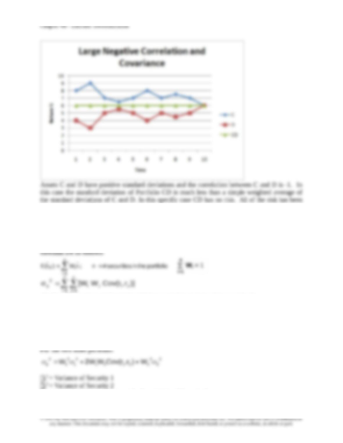
fall on a straight line because in this case p = Wii. However if the assets are perfectly
negatively correlated, we can combine the two securities to completely eliminate variance in
equations:
6-4
Chapter 06 – Efficient Diversification
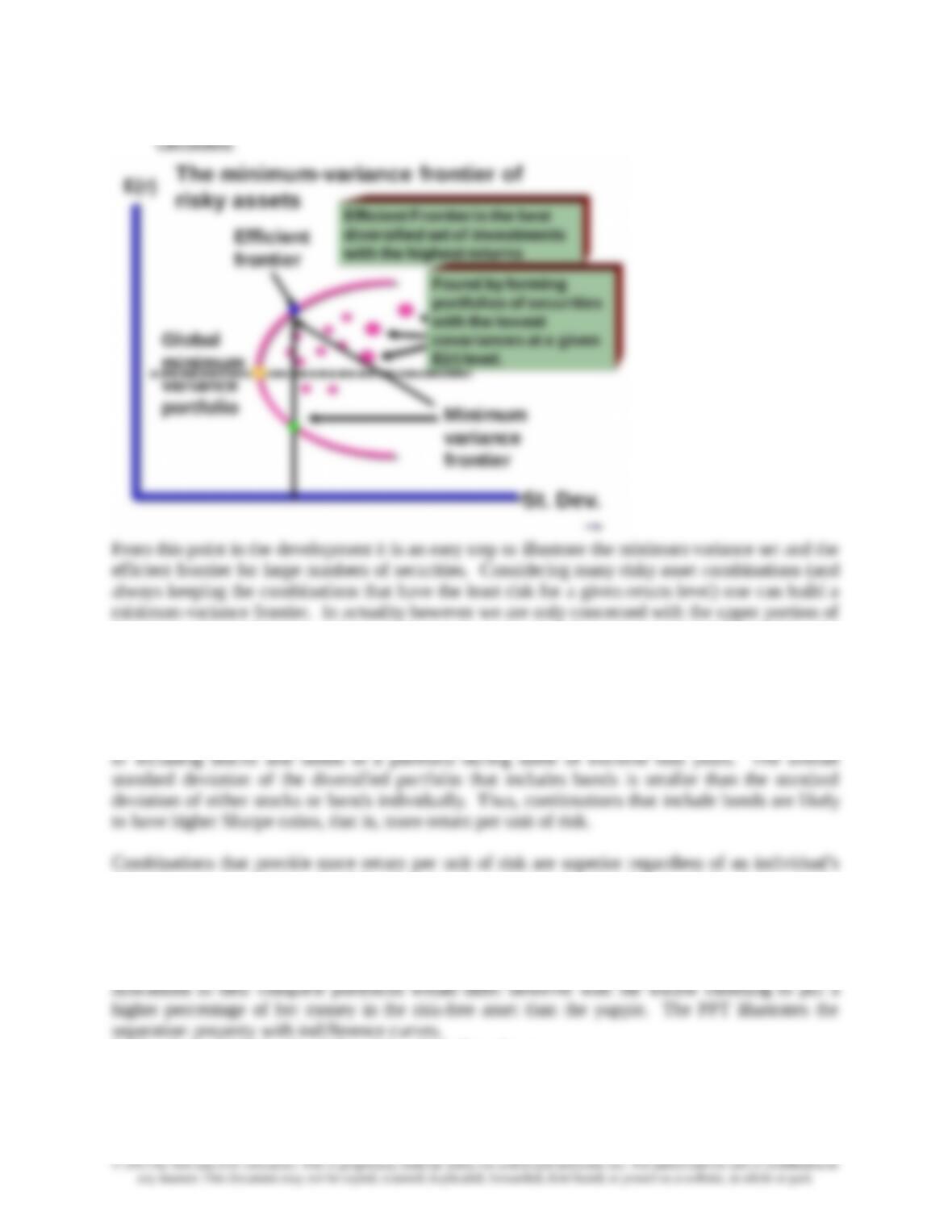
Once the weights are known, the minimum variance portfolio expected return and risk can be
the curve. Any minimum variance point on the bottom of the curve can be dominated by the
similar point on the upper portion of the curve. The curve from the global minimum–variance
portfolio, up and to the right, represents the efficient frontier, which are the best diversified
combinations or the least risky for each possible expected return level.
The text also illustrates the benefits of diversification, using historical data to examine the effects
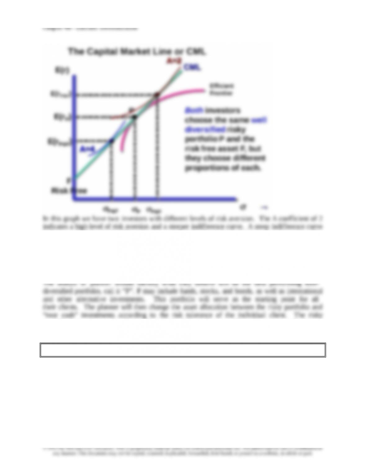
risk tolerance due to the principle of separation which holds that that portfolio choice can be
separated into two independent tasks: (1) determination of the optimal risky portfolio and (2) the
personal choice of the best mix of the risky portfolio and the risk free asset. This is a crucial
point. It means that a widow (with high risk aversion) and a ‘yuppie’ (a young upwardly mobile
professional with low risk aversion) should both choose the same risky portfolio. Their asset
3. The Optimal Risky Portfolio with a Risk-Free Asset
6-5
4. Efficient Diversification with Many Risky Assets
PPT 6-18 through PPT 6-29
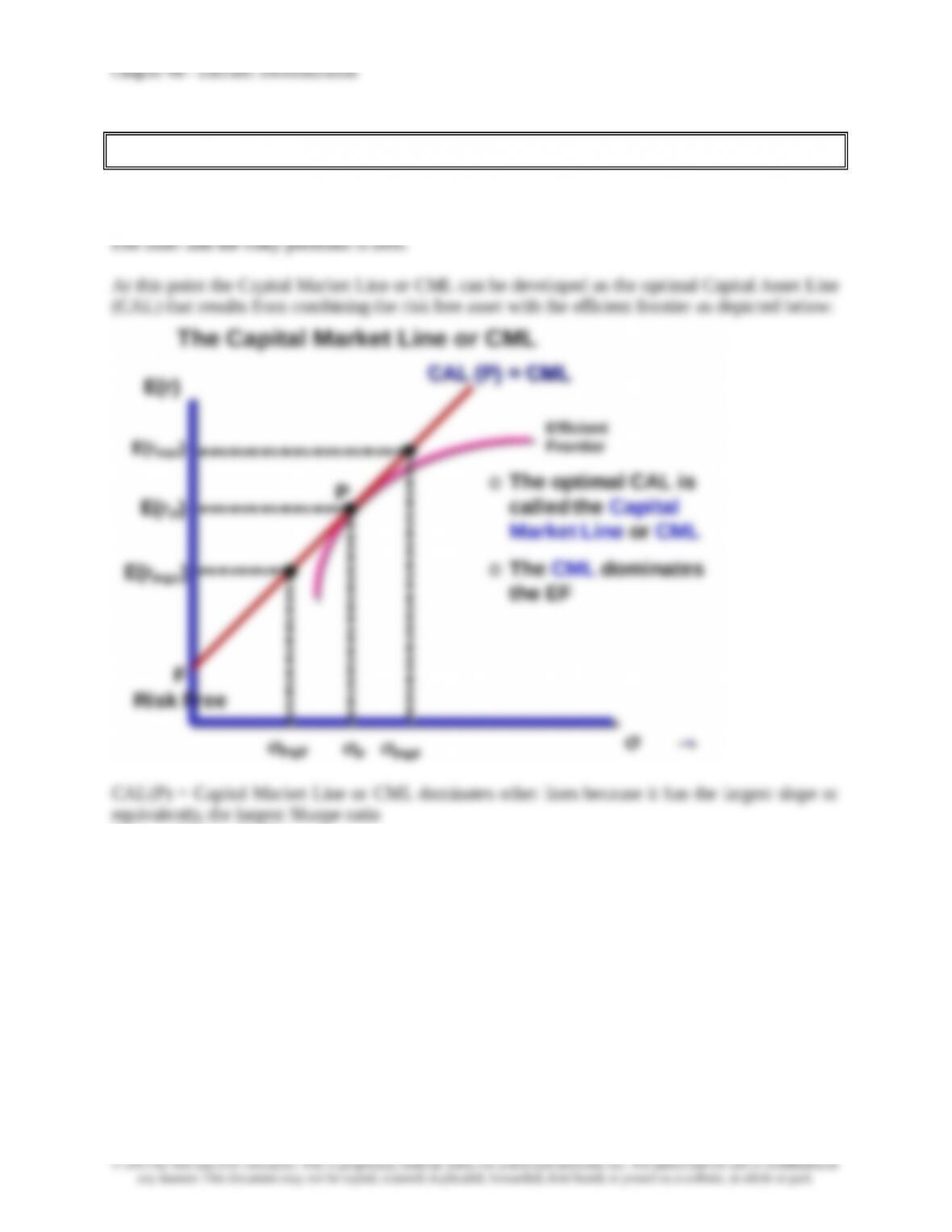
The inclusion of a risk-free asset in a portfolio results in a single combination of stock and bonds
that is optimal when that portfolio is combined with the risk-free asset. As explained in Chapter 5
the resulting capital allocation line is now linear. This is because the covariance between the risk
Slope = (E(rp) – rf) / p
That is, the CML maximizes the slope or the return per unit of risk or it equivalently maximizes
the Sharpe ratio. Regardless of risk preferences, some combinations of risky portfolio P & and
risk-free asset F will dominate all other combinations. All investors’ complete portfolio will fall on
the CML.
6-6
indicates a high level of additional return required by the individual investor to bear risk. The
slope of the indifference curve is the marginal rate of substitution (MRS). The slope of the CML
is the marginal rate of transformation (MRT). The optimal complete portfolio is found on the
CML where the MRS = MRT.
Practical Implications
portfolio P may have to be adjusted for individual clients for tax and liquidity concerns, if relevant,
and to adjust for the client’s unique circumstances.
5. A Single Index Asset Market
PPT 6-30 through PPT 6-38
We have learned that investors should diversify, thus individual securities will be held in a
portfolio.
6-7
in interest rates or GDP; or a financial crisis such as that which occurred in 2007 and 2008. If a
well diversified portfolio has no unsystematic risk then any risk that remains must be systematic;
the variation in returns of a well–diversified portfolio must be due to changes in systematic factors.
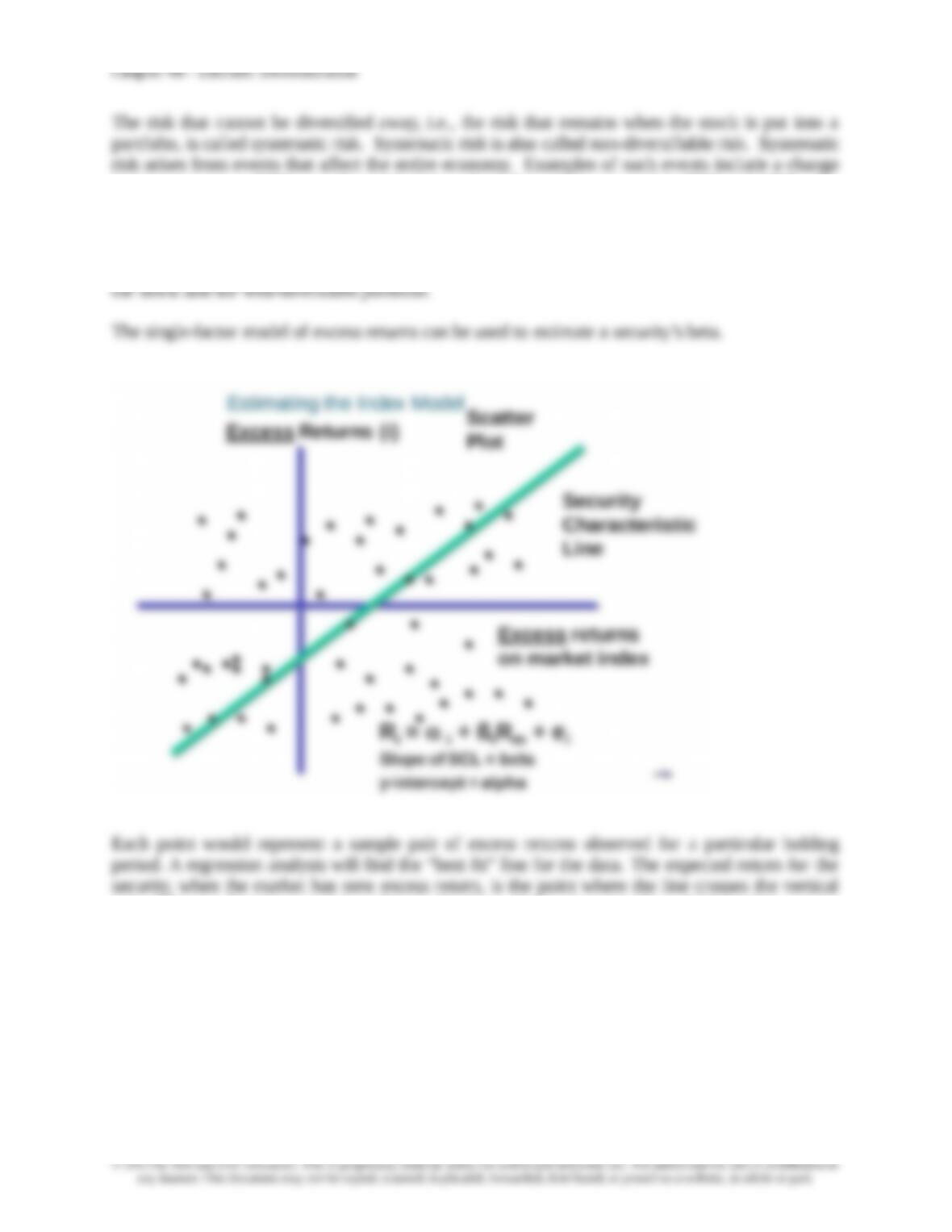
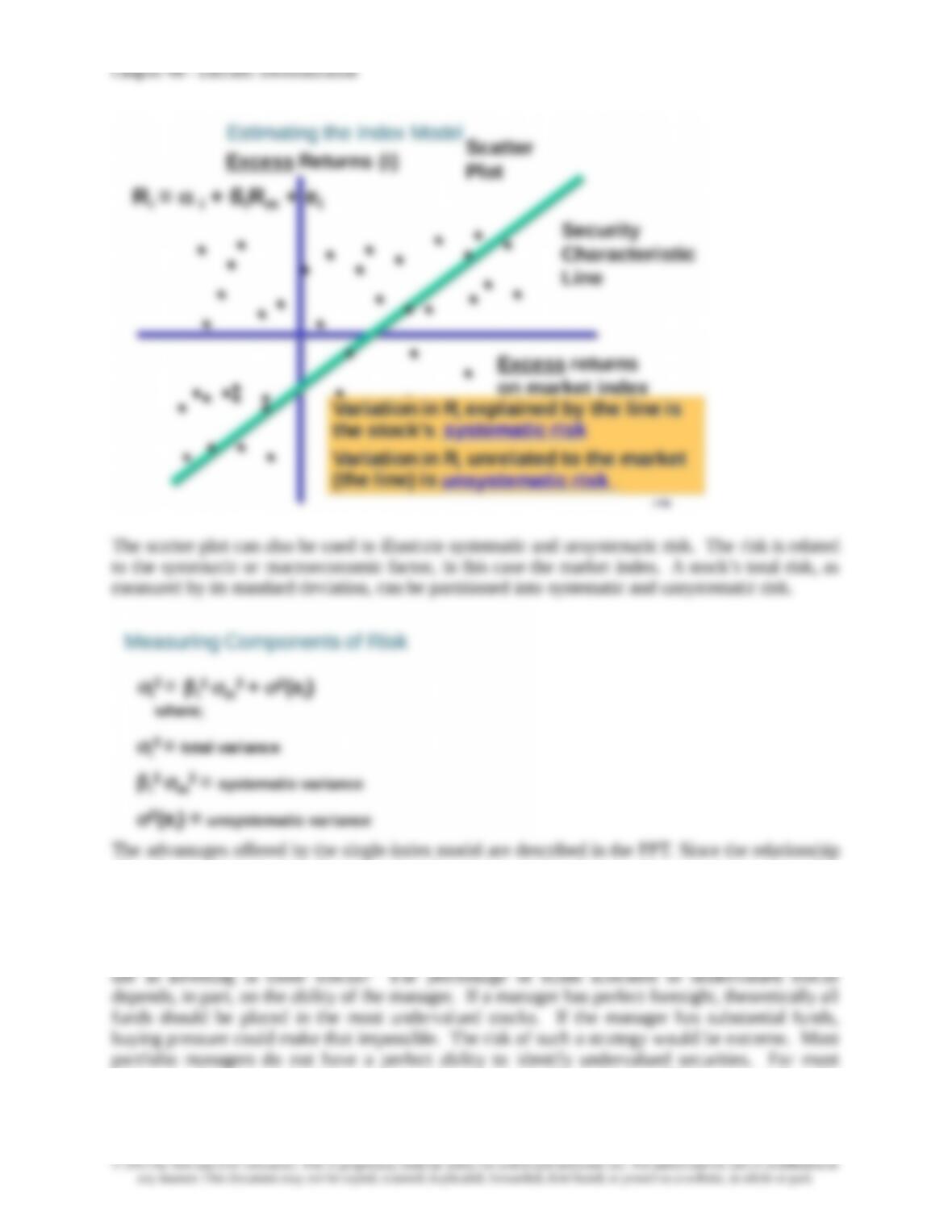
We have already learned that covariance is the predominant statistic in determining the risk of a
portfolio. Similarly, the systematic risk of an individual stock is a function of the covariance of
axis. This is referred to as alpha. Beta is the slope of the regression line. A higher beta means
higher systematic risk. Betas above 1 are riskier than the market since a regression of the market
excess returns versus market excess returns would, by definition, yield a beta of 1.
6-8
of each security is compared or related to the common index, data requirements are much smaller
than they would be if each pair-wise correlation was measured. Betas also provide an easy
reference point since the market beta is 1.
The Treynor-Black Model (advanced topic)
If a manager has the ability to find undervalued stocks, what strategy should a portfolio manager
managers, the process involves some passive investment in stocks in addition to acquiring the
undervalued stocks.
6-9

Chapter 06 – Efficient Diversification
portfolio is its ratio of alpha to nonsystematic risk.
By combining the active and passive portfolios, the manager can achieve a superior reward-to–risk
combination. Understanding the results of the Treynor-Black Model is best accomplished through
a graphical presentation. A graph is provided in the PPT. The standard Capital Market Line
(CML) is shown in the graph. The portfolio of actively managed stocks is shown as point A.
alpha in relation to the stock’s unsystematic risk. Suppose an investor holds a passive portfolio M
but believes that an individual security has a positive alpha. A positive alpha implies the security is
undervalued. Suppose Google has the positive alpha. Adding Google moves the overall portfolio
away from the diversified optimum, thus bearing residual risk that could be eliminated; however, it
might be worth it to earn the positive alpha. We need to determine the optimal portfolio including
• The improvement in the Sharpe ratio (S) over the Sharpe of the passive portfolio M can be
found as:
• This ratio is called the “information ratio.”
• For multiple stocks in the active portfolio:
6-10
PassiveM Google, G W1 W;
)β(1W1
W*
G
*
M
G
O
G
G
*
G
2
G
G
2
M
2
O)σ(e
α
SS
;
)σ(e
G
ii
2
i
i
2
i
*
i
)e(
)e(
W
)e(
…
)e()e()e( n
2
n
2
2
2
1
2
1
n
ii
2
i
6. Risk of Long-Term Investments
PPT 6-39 through PPT 6-40
The last section of this chapter provides a comparison of the variance and standard deviation of
short-term and long-term investments. PPT 6-41 and PPT 6-42 present a calculation for variance
iA
n
i
iAAiA
n
i
iAA W ; αWα
2
iA
n
i
2
iAA
2W)e(