Chapter 05 – Risk and Return: Past and Prologue
CHAPTER FIVE
RISK AND RETURN: PAST AND PROLOGUE
CHAPTER OVERVIEW
should be able to construct portfolios of different risk levels, given information about risk free
rates and returns on risky assets. The student should be able to calculate the expected return and
standard deviation of these combinations.
Students will learn that theoretically one can easily construct portfolios of varying degrees of risk
1. Rates of Return
PPT 5-2 through PPT 5-6
The PPT begins by calculating holding period returns or HPRs and discusses why we calculate
returns and sometimes annualize them. Annualizing with and without compounding is illustrated.
performance over the time under evaluation. Once the return series is calculated, either a
geometric or an arithmetic average may be calculated. Dollar-weighted returns include the effects
of the investor’s choices of when they bought and sold securities. Thus dollar-weighted returns
give the investor a truer estimate of the rate of return they earned based on security return
performance and their own choices of when they bought and sold the security.
2. Risk and Risk Premiums
PPT 5-6 through PPT 5-14
This section begins by illustrating calculations of expected returns and standard deviation ex-ante
for individual securities via scenario analysis. Ex-post average return and standard-deviation
calculations are also provided. Basic characteristics of probability distributions are then covered
How many dollars can I expect to lose on my portfolio in a given time period at a given level of
probability?
The typical probability used is 5%.
In a given probability distribution we need to know what HPR corresponds to a 5% probability.
If returns are normally distributed then we can use a standard normal table or Excel to determine
VaR = E[r] + -1.64485s \
For Example:
A $500,000 stock portfolio has an annual expected return of 12% and a standard deviation of
35%. What is the portfolio VaR at a 5% probability level?
VaR = 0.12 + (-1.64485 * 0.35)
normal distributions. The text illustrates calculating VaR if you have a normal distribution. If
options or other complex instruments are included in the portfolio you will not have a normal
distribution. You then have to approximate the distribution or perhaps use a Monte Carlo
simulation to build a distribution of future returns.
5-2
distributions are not normally distributed. Note the actual 5% probability level will differ from
1.68445 standard deviations from the mean due to kurtosis and skewness if these are present. In
these cases the standard deviation is a not a sufficient statistic to measure risk.
Risk Premium and Risk Aversion
3. The Historical Record
PPT 5-15 through PPT 5-16
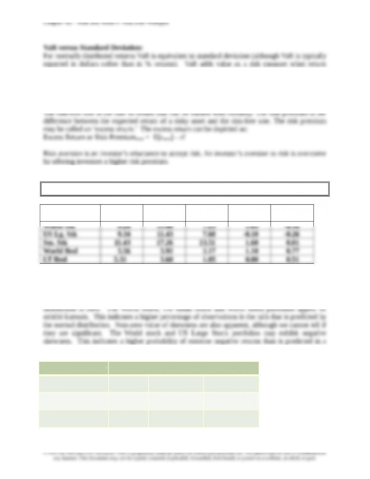
Annual Holding Period Returns Statistics 1926-2008 (From Table 5.3)
Geom.
Mean%
Arith.
Mean%
Excess
Return% Kurt. Skew.Series
The geometric mean is the best measure of the compound historical rate of return. Nevertheless
the arithmetic average is the best measure of the expected return. Notice the greater divergence
of the GAR and AAR for small stocks. This is because of the high variance and the higher
proportion of negative returns in the small stock portfolio. Although we don’t have statistical
significance it appears that some of the portfolios exhibit kurtosis. Kurtosis of the normal
normal distribution.
Portfolio
World Stock US Small Stock US Large Stock
Arithmetic Average .1100 .1726 .1143
Geometric Average .0920 .1143 .0934
5-3
Variance .0186 .0694 .0214
If returns are normally distributed then the following relationship among geometric and arithmetic
averages holds:
Arithmetic Average – Geometric Average = ½ s2
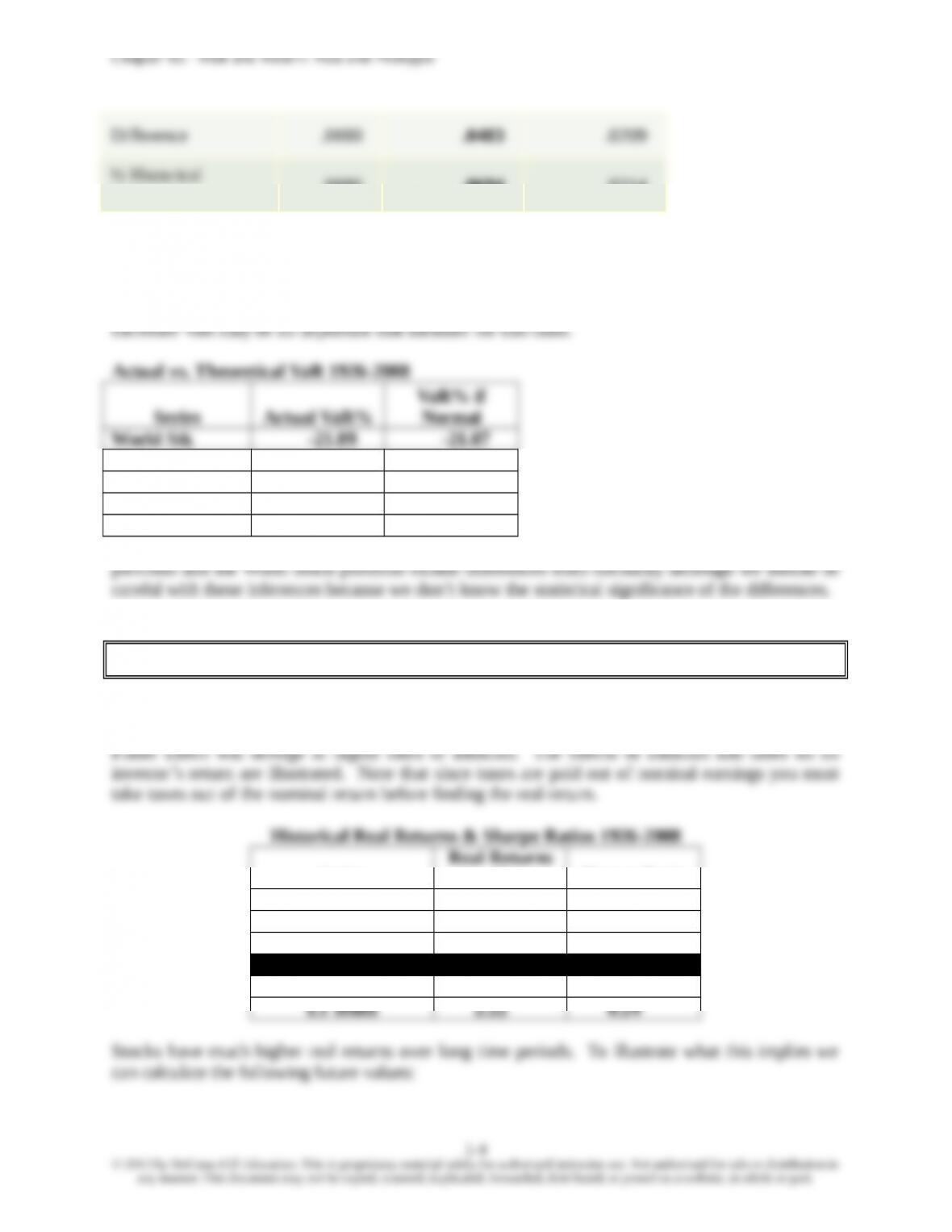
The comparisons above indicate that US Small Stocks may have deviations from normality and
US Lg. Stk -29.79 -22.92
Sm. Stk -46.25 -44.93
World Bnd -6.54 -8.69
LT Bnd -7.61 -7.25
These comparisons may indicate that the U.S. Large Stock portfolio, the US Small Stock
4. Inflation and Real Rates of Return
PPT 5-17 through PPT 5-19
The concept of real versus nominal rates and the Fisher Effect are presented. The reason for
needing the exact version of the Fisher Effect is given in a hidden slide with a hyperlink so that the
instructor may use it or not. Note that the approximation version and the exact version of the
Series
% Sharpe Ratio
World Stk 6.00 0.37
US Lg. Stk 6.13 0.37
Sm. Stk 8.17 0.36
World Bnd 2.46 0.24
Chapter 05 – Risk and Return: Past and Prologue
LT Bond portfolio: $1 x 1.02282 = $5.96; if you had invested $1 in the LT Bond portfolio for 82
years your $1 would have grown to the equivalent purchasing power of just under $6.
US Large Stock portfolio: $1 x 1.0682 = $118.87; if you invested $1 in the US Large Stock
portfolio for 82 years your $1 would have grown to the equivalent purchasing power of just under
should not hold bonds? No, adding bonds to a stock portfolio will eliminate proportionally more
risk than the return sacrificed and can lead to higher Sharpe ratios.
5. Asset Allocation across Risky and Risk-Free Portfolios
PPT 5-20 through PPT 5-24
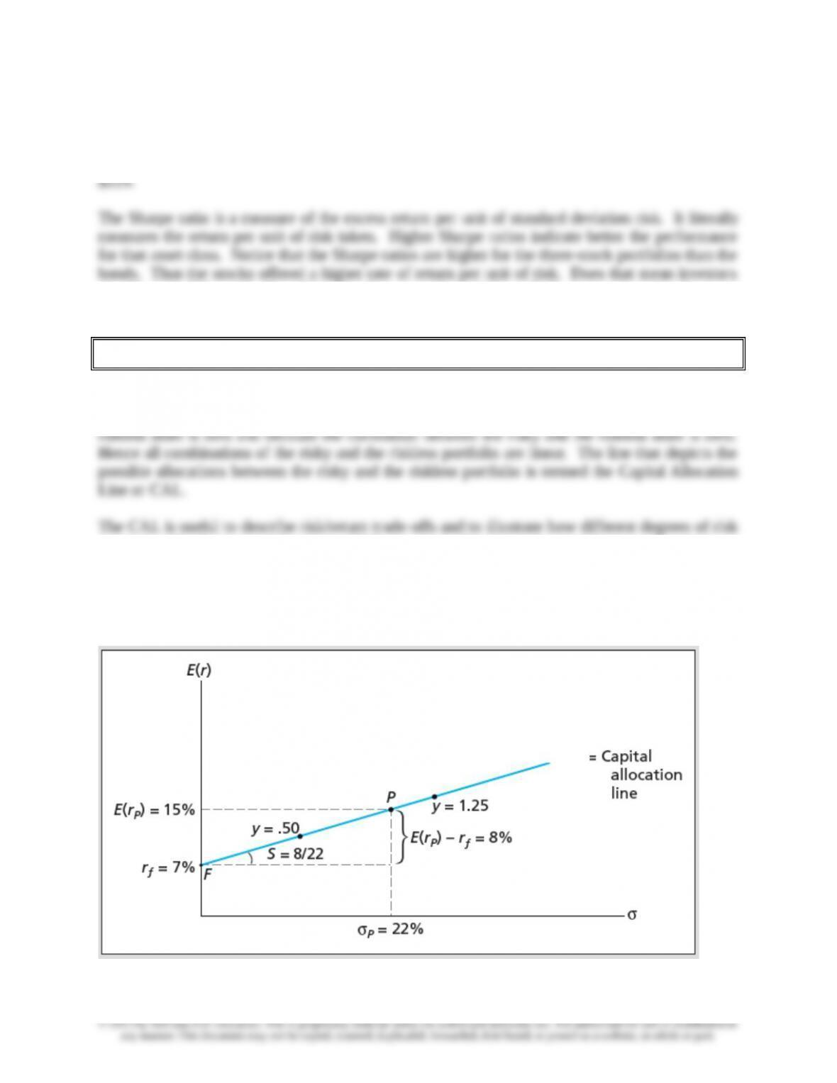
Investors can choose to hold risky and riskless assets. We may consider investments in a money
market mutual fund as a proxy for the riskless investments that an investor might actually engage
in. These combinations fall on a straight line (see below) because the standard deviation of the
aversion will affect asset allocation. Risk aversion will impact the combinations chosen by an
investor. An investor with a low tolerance for risk will likely prefer to invest some funds in the
risk-less asset. An investor with a high tolerance for risk may choose to use leverage.
Understanding the CAL now will help students understand the modeling in the next chapter when
we consider multiple risky asset combinations.
5-5
CAL
a zero standard deviation. With 100% of your money in the risky asset you will have a 15%
expected return and a 22% standard deviation. Combinations (y) less than one represent varying
percentages invested in the risky asset P and (1-y) the percentage invested in the risk free F.
Combinations above P are possible by borrowing money at F. This is conceptually equivalent to
buying stock on margin. More risk-averse investors would choose a lower y and less risk-averse
2
p
fp A5.0rrE
E(rp) = Expected return on portfolio p
rf = the risk free rate
0.5 = Scale factor
A x sp2 = Proportional risk premium
A larger A indicates that the investor requires more return to bear risk. In the asset allocation
decision the optimal weight in the risky portfolio P (WP) is:
2
P
fP
pA
r)r(E
w
The coefficient of risk aversion A is generally thought to be between 2 and 4.
With an assumed utility function of the form:
U = E[r] – 1/2Asp2
The A term can used to create indifference curves. Indifference curves describe different
combinations of return and risk that provide equal utility (U) or satisfaction. Indifference curves
are curvilinear because they exhibit diminishing marginal utility of wealth. The greater the A the
steeper the indifference curve and all else equal, such investors will invest less in risky assets. The
smaller the A the flatter the indifference curve and all else equal, such investors will invest more in
risky assets.
6. Passive Strategies and the Capital Market Line
PPT 5-25 through PPT 5-27
In a passive strategy the investor makes no attempt to either find undervalued strategies or
actively switch their asset allocations. Investing in a broad stock index and a risk-free investment
is an example of a passive strategy. The CAL that employs the market (or an index that mimics
Excess Returns and Sharpe Ratios Implied by the CML
Excess Return or Risk
Premium
Time Period Average Sharpe
5-6

1956-1984 5.01 17.58 0.28
1985-2008 5.95 18.23 0.33
The average risk premium implied by the CML for large common stocks over the entire time
period is 7.86%. But the subperiod variation and the large standard deviation indicate that
investors cannot be very confident about using the historical data to estimate what the risk