Chapter 15
Independent Demand Inventory
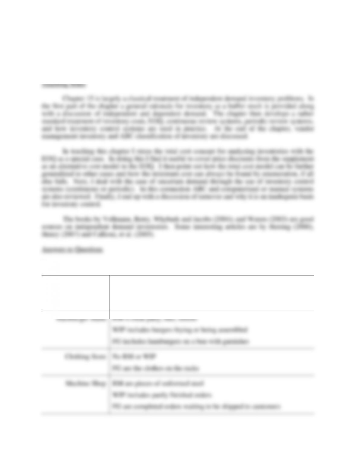
1.
Gas Station
No RM or WIP
Finished goods include gas, oil, tires, other car parts plus food and
general store items
Hamburger Stand
RM is meat patty, bun, onions
WIP includes burgers frying or being assembled
FG includes hamburgers on a bun with garnishes
Clothing Store
No RM or WIP
FG are the clothes on the racks
Machine Shop
RM are pieces of unformed steel
WIP includes partly finished orders
FG are completed orders waiting to be shipped to customers
the first part of the chapter a general rationale for inventory as a buffer stock is provided along
standard treatment of inventory costs, EOQ, continuous review systems, periodic review systems,
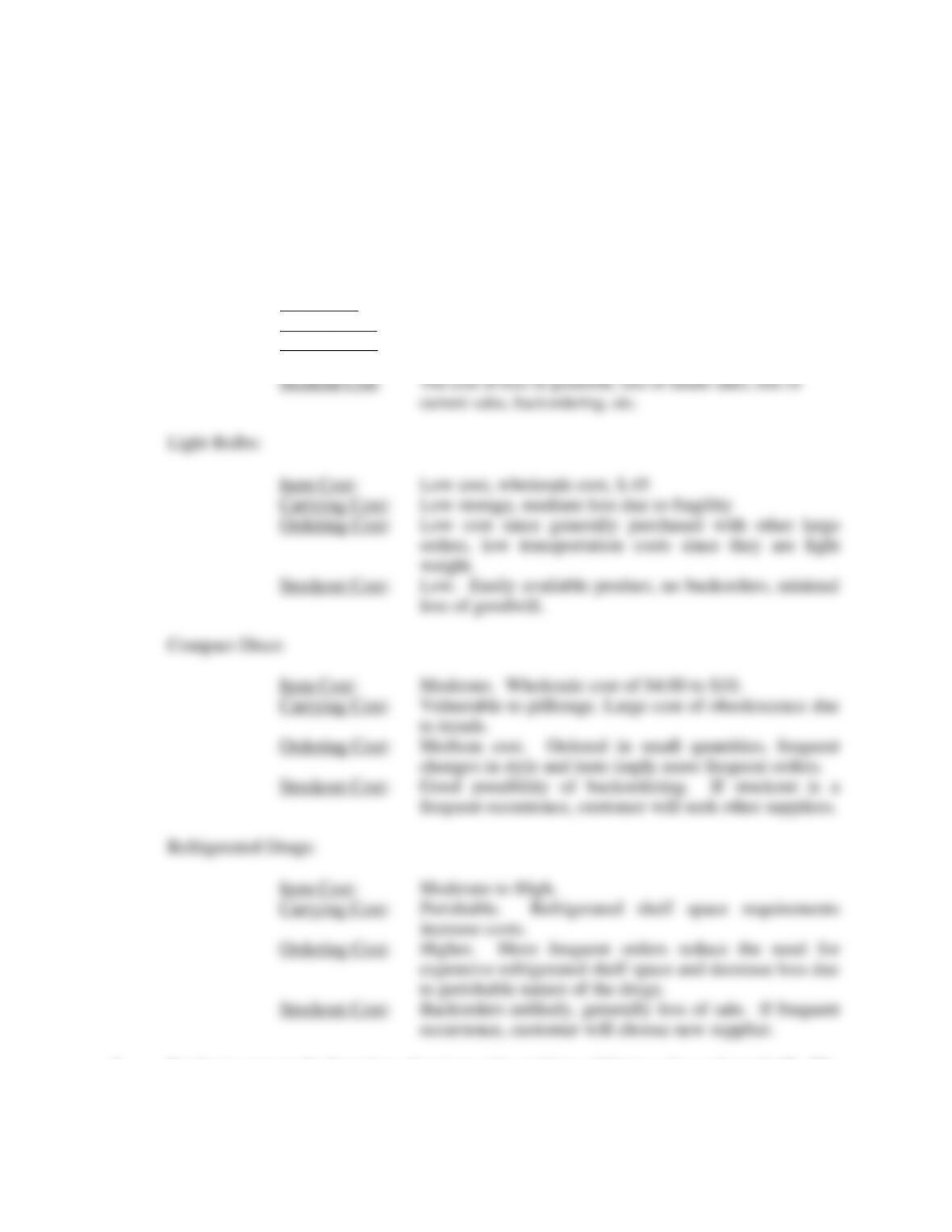
2. General:
Item Cost: The cost of buying or producing the product
Carrying Cost: The cost of storage, loss, facilities, and capital
Ordering Cost: The cost of negotiating with vendors, writing and processing
the order, receiving inspection, transportation, etc.
3. Stockout cost results from loss of current sales and loss of future sales and goodwill. The
profit foregone from loss of current sales can be estimated; lost future sales and goodwill,
however, implies an opportunity loss for which historical data is of little help.
One approach to estimation of stockout cost might be to sum the estimated profit from
current sales lost (average daily profit per item x number of days until available) and an
4. Item cost is assumed to be constant with no quantity discounts. Since item cost does not
depend on Q, the quantity ordered, the item cost does not affect the minimum of the cost
equation.
Item cost is important in EOQ calculations when there are quantity discounts because a
lower unit price is usually offered in return for larger lot sizes. In this case the cost of the
5. A requirements philosophy of inventory management is appropriate when demand is
dependent; a replenishment philosophy is appropriate given independent demand. The
requirements philosophy calls for orders based on requirements for higher-level items. The
replenishment philosophy relates demand to the market.
The difference is important since the philosophy toward inventory influences the type of
6. Manufacturing has three different types of inventory to manage: raw materials, work in
process, and finished goods. The demand for raw materials and WIP is dependent on the
demand for finished goods. The requirements philosophy is used to avoid shortages in raw
materials or WIP which can hold up the entire production process. Manufacturing must
forecast independent demand for finished products that will drive the requirements for WIP
and raw materials.
7. Due to the need to review stock position at fixed intervals, a target level of stock must be
ordered to cover demand until the next review period. This estimated amount is over and
above the amount required to cover just lead time. The target is calculated as “m’ + s'”
where m’ (average demand over P + L) is greater than m and where s’, safety stock for P +
L, is greater than s. Factors affecting the magnitude of the difference in inventory
investment are the same factors which affect safety stock. The difference in safety stock
8. In a hardware store, the P system might be used for nails or screws in bins, screwdrivers,
hammers, and garden hand tools. This is because these items have a lower unit cost, lower
carrying costs, lower ordering costs, and higher turnover in the store. The Q system might
be used for power tools, small appliances, and power lawn equipment. This is because
these items have a higher unit costs, higher stockout costs, higher carrying costs, and higher
ordering costs.
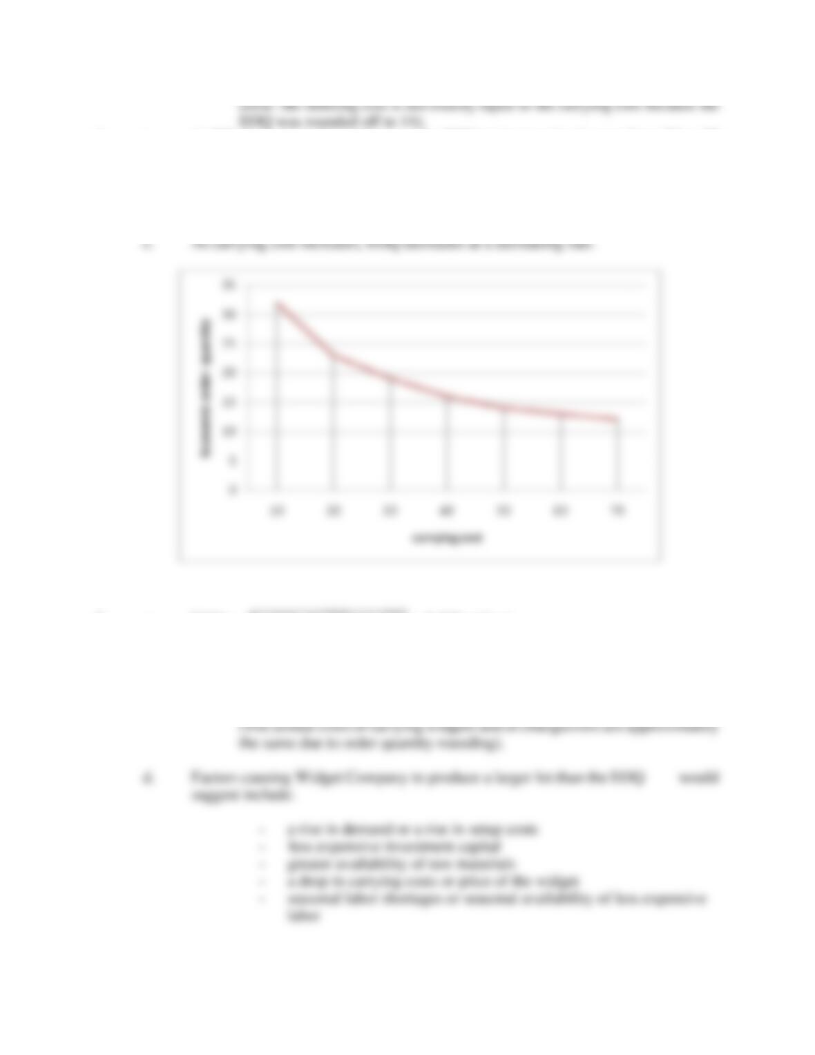
9. A decision on customer service level must consider the critical tradeoff between customer
satisfaction and inventory level, i.e., between inventory carrying costs and the cost of lost
sales and goodwill from customer dissatisfaction. The manager might try to evaluate this
tradeoff by first plotting various service levels against the inventory level required to
sustain each level of service. Viewing this nonlinear curve, the manager can see at which
level of service inventory costs begin to rise at an increasing rate. Also to be considered
10. The problem is that orders are being placed using on-hand inventory, when both on-hand
and on-order quantities should be used. Ignoring on-order material has the effect of
increasing order placement and inventories.
11. Even though the EOQ assumptions are restrictive, the EOQ formula is a useful
approximation in practice. Since the total inventory cost curve is rather flat in the region
of the minimum, order size can be adjusted somewhat without greatly affecting the costs.
For example, the model is fairly insensitive to changes in the ordering and carrying costs.
Order size may vary somewhat to reflect demand fluctuations without a large effect on total
costs.
12. Contrary to traditional arguments, inventory should not increase directly with sales to
maintain a constant turnover ratio. The EOQ formula is useful in showing that inventory
should increase only with the square root of sales. With very high sales, inventory may
increase at a slower rate and a higher turnover is justified. The turnover ratio is an indicator
to be monitored and should not form the only basis for inventory policies. High turnover
can be detrimental when it has risen steeply, indicating not a boost in sales but a reduction
13. Having set an overall company inventory policy including service level standards for each
product group in a store:
a. Verify that service level was met over the period using data on backorders,
stockouts, and complaints.
1. a. EOQ = 2SD/iC = 2(10)(416)/.2(80) = 22.8 23 cases
b. 23/8 = 2.8 so order every 2.8 weeks
416 cases/year 23 = 18.1 so order 18.1 times per year
c. Annual ordering cost = SD/Q = (10)(416)/23 = $ 180.8
Annual carrying cost = iCQ/2 = .2(80)(23)/2 = $ 184
(note: these costs are not exactly equal due to roundoff of EOQ)
2. a. EOQ = 2(1200)(300)/.2(25) 379 tables
b. 300/379 = 0.79, set up production 0.79 times per year
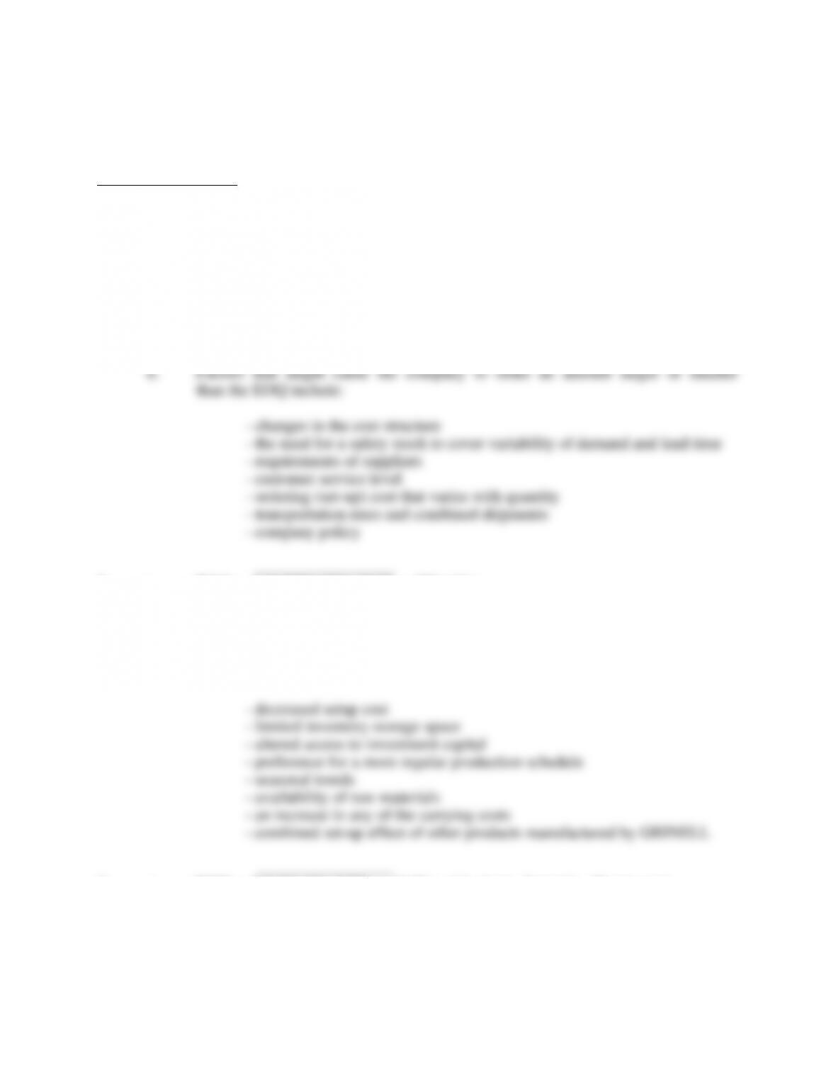
c. The company might schedule a different lot size, say 300 tables to be
produced say once per year, due to factors such as:
3. a. EOQ = 2(15)(48)/.3(25) = (note: demand = 48 per year)
b. 48/14 = 3.43 reorder times per year
c. Annual ordering cost = SD/Q = (15)(48)/14 = $51.43
Annual carrying cost = iCQ/2 = .3(25)(14)/2 = $52.50
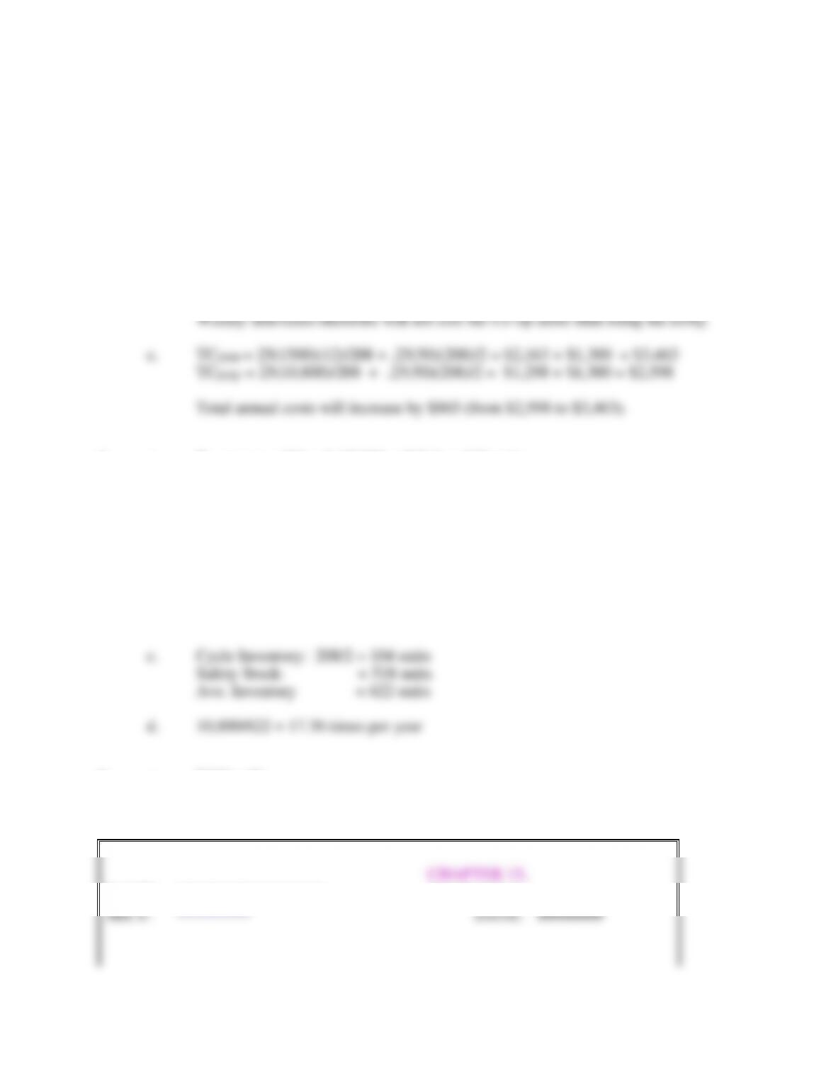
4. a. A 40% increase in demand causes the EOQ to increase by 4 cases from 23 to 27
cases, and total cost to increase by $67 from $365 to $432 per year.
b. A 20% increase in carrying costs causes EOQ to decrease by 2 cases from 23 to 21
cases, and total cost to increase by $35 from $365 to $400 per year.
5. a. EOQ = 2(1000)(80,000)/.3(100) 2,309 widgets
b. 80,000/2309 = 34.65 lots per year
c. Annual carrying cost = iCQ/2 = .3(100)2309/2 = $34,635
Annual ordering cost = SD/Q = 1000(80000)/2309 = $34,647
6. a. EOQ = 2(25)(10,800)/.25(50) = 207.85 208 (note: demand = 10,800 per
year)
b. Lot size of (10,800 52) 208
The weekly delivery quantity required is by coincidence just equal to the EOQ.
7. a. R = m + s = 450 + (1.65)250 = 862.5 863 units
b. Number of orders placed per year = 10,800/208 52
1/52 = 0.01923
One stockout per year is equivalent to a service level of 1-0.01923 =98.07%. Thus
use z = 2.07
R = 450 + (2.07)250 = 450 + 517.5 = 967.5 968 units
8. a. EOQ = 26
b. Reorder Point = 23.6
NAME:
******************
CHAPTER 15,
PROBLEM 8
SECT:
*********
DATE:
########
INPUT SECTION:
OUTPUT SECTION:
*
*
*
*
*
*
*
ANNUAL SALES:
1440
EOQ =
26
ORDERING COST:
$25
REORDER
POINT=
23.6
CARRYING COST
(%):
35%
z =
1.41
ITEM COST:
$300
ORDER
EVERY:
4.5
DAYS
STANDARD
DEVIATION:
0.2
*
*
*
*
WORKING
DAYS/YEAR:
250
LEAD TIME
(DAYS):
4
SERVICE LEVEL:
92%
*
*
*
9. a. P is 4.55 days and T is 50 units.
NAME:
******************
CHAPTER 15
PROBLEM 9
SECT:
******************
DATE:
########
PART A
ANNUAL SALES:
1440
ORDERING COST:
$25
CARRYING COST (%):
35%
INPUT
ITEM COST:
$300
SECTION
STD DEV.
0.2
WORKING DAYS/YEAR:
250
LEAD TIME:
4
SERVICE LEVEL:
92%
2. General:
Item Cost: The cost of buying or producing the product
Carrying Cost: The cost of storage, loss, facilities, and capital
Ordering Cost: The cost of negotiating with vendors, writing and processing
the order, receiving inspection, transportation, etc.
3. Stockout cost results from loss of current sales and loss of future sales and goodwill. The
profit foregone from loss of current sales can be estimated; lost future sales and goodwill,
however, implies an opportunity loss for which historical data is of little help.
One approach to estimation of stockout cost might be to sum the estimated profit from
current sales lost (average daily profit per item x number of days until available) and an
4. Item cost is assumed to be constant with no quantity discounts. Since item cost does not
depend on Q, the quantity ordered, the item cost does not affect the minimum of the cost
equation.
Item cost is important in EOQ calculations when there are quantity discounts because a
lower unit price is usually offered in return for larger lot sizes. In this case the cost of the
5. A requirements philosophy of inventory management is appropriate when demand is
dependent; a replenishment philosophy is appropriate given independent demand. The
requirements philosophy calls for orders based on requirements for higher-level items. The
replenishment philosophy relates demand to the market.
The difference is important since the philosophy toward inventory influences the type of
6. Manufacturing has three different types of inventory to manage: raw materials, work in
process, and finished goods. The demand for raw materials and WIP is dependent on the
demand for finished goods. The requirements philosophy is used to avoid shortages in raw
materials or WIP which can hold up the entire production process. Manufacturing must
forecast independent demand for finished products that will drive the requirements for WIP
and raw materials.
7. Due to the need to review stock position at fixed intervals, a target level of stock must be
ordered to cover demand until the next review period. This estimated amount is over and
above the amount required to cover just lead time. The target is calculated as “m’ + s'”
where m’ (average demand over P + L) is greater than m and where s’, safety stock for P +
L, is greater than s. Factors affecting the magnitude of the difference in inventory
investment are the same factors which affect safety stock. The difference in safety stock
8. In a hardware store, the P system might be used for nails or screws in bins, screwdrivers,
hammers, and garden hand tools. This is because these items have a lower unit cost, lower
carrying costs, lower ordering costs, and higher turnover in the store. The Q system might
be used for power tools, small appliances, and power lawn equipment. This is because
these items have a higher unit costs, higher stockout costs, higher carrying costs, and higher
ordering costs.
9. A decision on customer service level must consider the critical tradeoff between customer
satisfaction and inventory level, i.e., between inventory carrying costs and the cost of lost
sales and goodwill from customer dissatisfaction. The manager might try to evaluate this
tradeoff by first plotting various service levels against the inventory level required to
sustain each level of service. Viewing this nonlinear curve, the manager can see at which
level of service inventory costs begin to rise at an increasing rate. Also to be considered
10. The problem is that orders are being placed using on-hand inventory, when both on-hand
and on-order quantities should be used. Ignoring on-order material has the effect of
increasing order placement and inventories.
11. Even though the EOQ assumptions are restrictive, the EOQ formula is a useful
approximation in practice. Since the total inventory cost curve is rather flat in the region
of the minimum, order size can be adjusted somewhat without greatly affecting the costs.
For example, the model is fairly insensitive to changes in the ordering and carrying costs.
Order size may vary somewhat to reflect demand fluctuations without a large effect on total
costs.
12. Contrary to traditional arguments, inventory should not increase directly with sales to
maintain a constant turnover ratio. The EOQ formula is useful in showing that inventory
should increase only with the square root of sales. With very high sales, inventory may
increase at a slower rate and a higher turnover is justified. The turnover ratio is an indicator
to be monitored and should not form the only basis for inventory policies. High turnover
can be detrimental when it has risen steeply, indicating not a boost in sales but a reduction
13. Having set an overall company inventory policy including service level standards for each
product group in a store:
a. Verify that service level was met over the period using data on backorders,
stockouts, and complaints.
1. a. EOQ = 2SD/iC = 2(10)(416)/.2(80) = 22.8 23 cases
b. 23/8 = 2.8 so order every 2.8 weeks
416 cases/year 23 = 18.1 so order 18.1 times per year
c. Annual ordering cost = SD/Q = (10)(416)/23 = $ 180.8
Annual carrying cost = iCQ/2 = .2(80)(23)/2 = $ 184
(note: these costs are not exactly equal due to roundoff of EOQ)
2. a. EOQ = 2(1200)(300)/.2(25) 379 tables
b. 300/379 = 0.79, set up production 0.79 times per year
c. The company might schedule a different lot size, say 300 tables to be
produced say once per year, due to factors such as:
3. a. EOQ = 2(15)(48)/.3(25) = (note: demand = 48 per year)
b. 48/14 = 3.43 reorder times per year
c. Annual ordering cost = SD/Q = (15)(48)/14 = $51.43
Annual carrying cost = iCQ/2 = .3(25)(14)/2 = $52.50
4. a. A 40% increase in demand causes the EOQ to increase by 4 cases from 23 to 27
cases, and total cost to increase by $67 from $365 to $432 per year.
b. A 20% increase in carrying costs causes EOQ to decrease by 2 cases from 23 to 21
cases, and total cost to increase by $35 from $365 to $400 per year.
5. a. EOQ = 2(1000)(80,000)/.3(100) 2,309 widgets
b. 80,000/2309 = 34.65 lots per year
c. Annual carrying cost = iCQ/2 = .3(100)2309/2 = $34,635
Annual ordering cost = SD/Q = 1000(80000)/2309 = $34,647
6. a. EOQ = 2(25)(10,800)/.25(50) = 207.85 208 (note: demand = 10,800 per
year)
b. Lot size of (10,800 52) 208
The weekly delivery quantity required is by coincidence just equal to the EOQ.
7. a. R = m + s = 450 + (1.65)250 = 862.5 863 units
b. Number of orders placed per year = 10,800/208 52
1/52 = 0.01923
One stockout per year is equivalent to a service level of 1-0.01923 =98.07%. Thus
use z = 2.07
R = 450 + (2.07)250 = 450 + 517.5 = 967.5 968 units
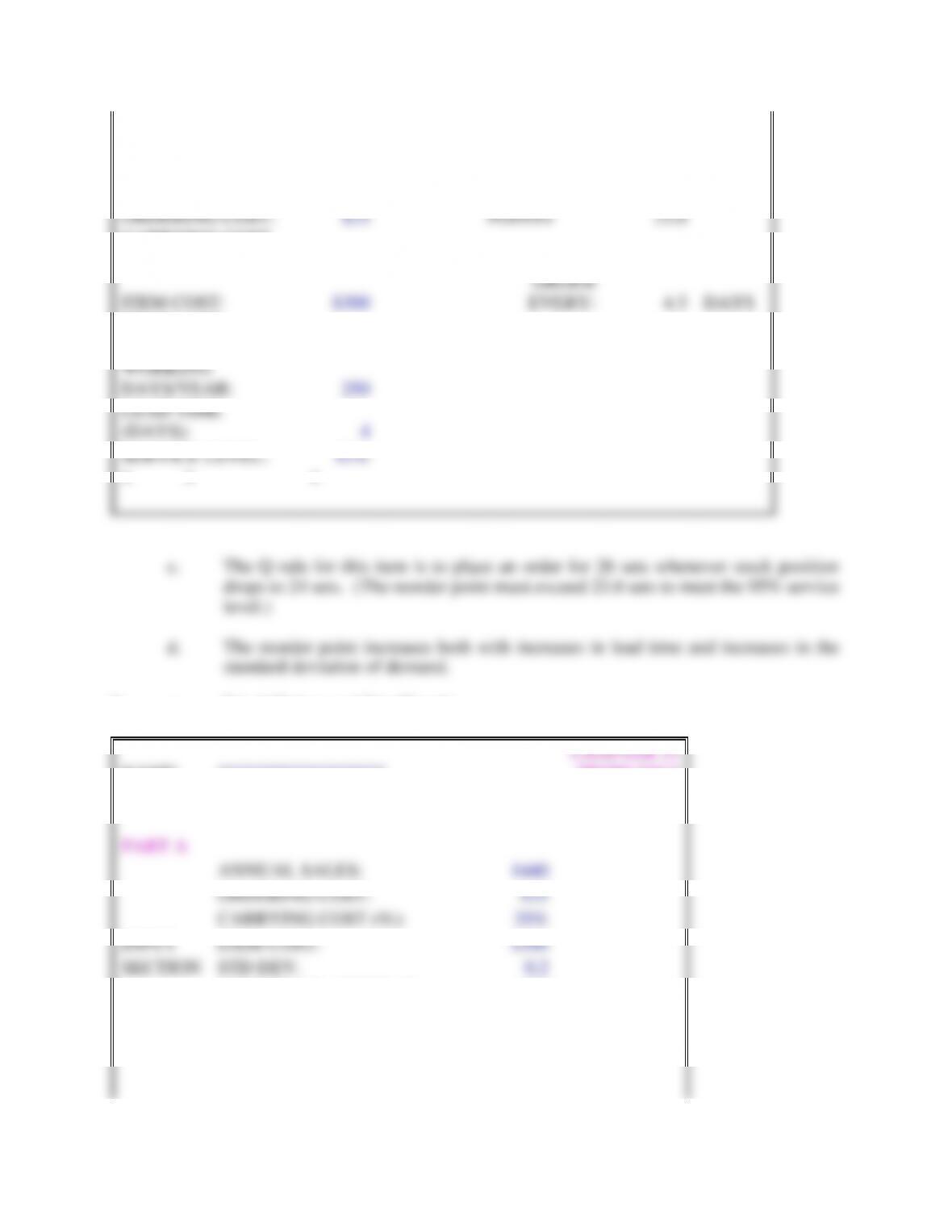
8. a. EOQ = 26
b. Reorder Point = 23.6
NAME:
******************
CHAPTER 15,
PROBLEM 8
SECT:
*********
DATE:
########
INPUT SECTION:
OUTPUT SECTION:
*
*
*
*
*
*
*
ANNUAL SALES:
1440
EOQ =
26
ORDERING COST:
$25
REORDER
POINT=
23.6
CARRYING COST
(%):
35%
z =
1.41
ITEM COST:
$300
ORDER
EVERY:
4.5
DAYS
STANDARD
DEVIATION:
0.2
*
*
*
*
WORKING
DAYS/YEAR:
250
LEAD TIME
(DAYS):
4
SERVICE LEVEL:
92%
*
*
*
9. a. P is 4.55 days and T is 50 units.
NAME:
******************
CHAPTER 15
PROBLEM 9
SECT:
******************
DATE:
########
PART A
ANNUAL SALES:
1440
ORDERING COST:
$25
CARRYING COST (%):
35%
INPUT
ITEM COST:
$300
SECTION
STD DEV.
0.2
WORKING DAYS/YEAR:
250
LEAD TIME:
4
SERVICE LEVEL:
92%