
53.3 52.3
= .3 produces the smaller absolute error and smaller tracking signal values.
= .1 = .3
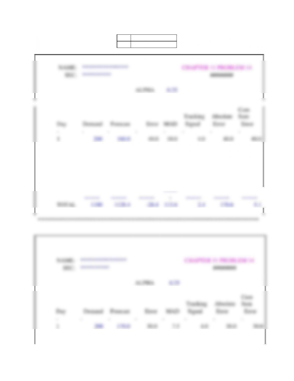
12. b. Day Dt Ft et MAD TS Ft et MAD TS
8 39 32.0 7.0 0.7 10.0 32.0 7.0 2.1 3.3
9 24 32.7 8.7 1.5 -1.1 34.1 10.1 4.5 -0.7
10 26 31.8 5.8 1.9 -3.9 31.1 5.1 4.7 -1.7
11 36 31.2 4.8 2.2 -1.3 29.5 6.5 5.2 -0.3
12 43 31.7 11.3 3.1 2.7 31.5 11.5 7.1 1.4
13 46 32.9 13.1 4.1 5.2 34.9 11.1 8.3 2.5
14 29 34.2 5.2 4.2 3.9 38.3 9.3 8.6 1.4
55.9 60.6
Now = .1 produces the smaller absolute error, and tracking signal results are
acceptable for both values of .
c. This example illustrates that variability in the data may cause some forecasting methods
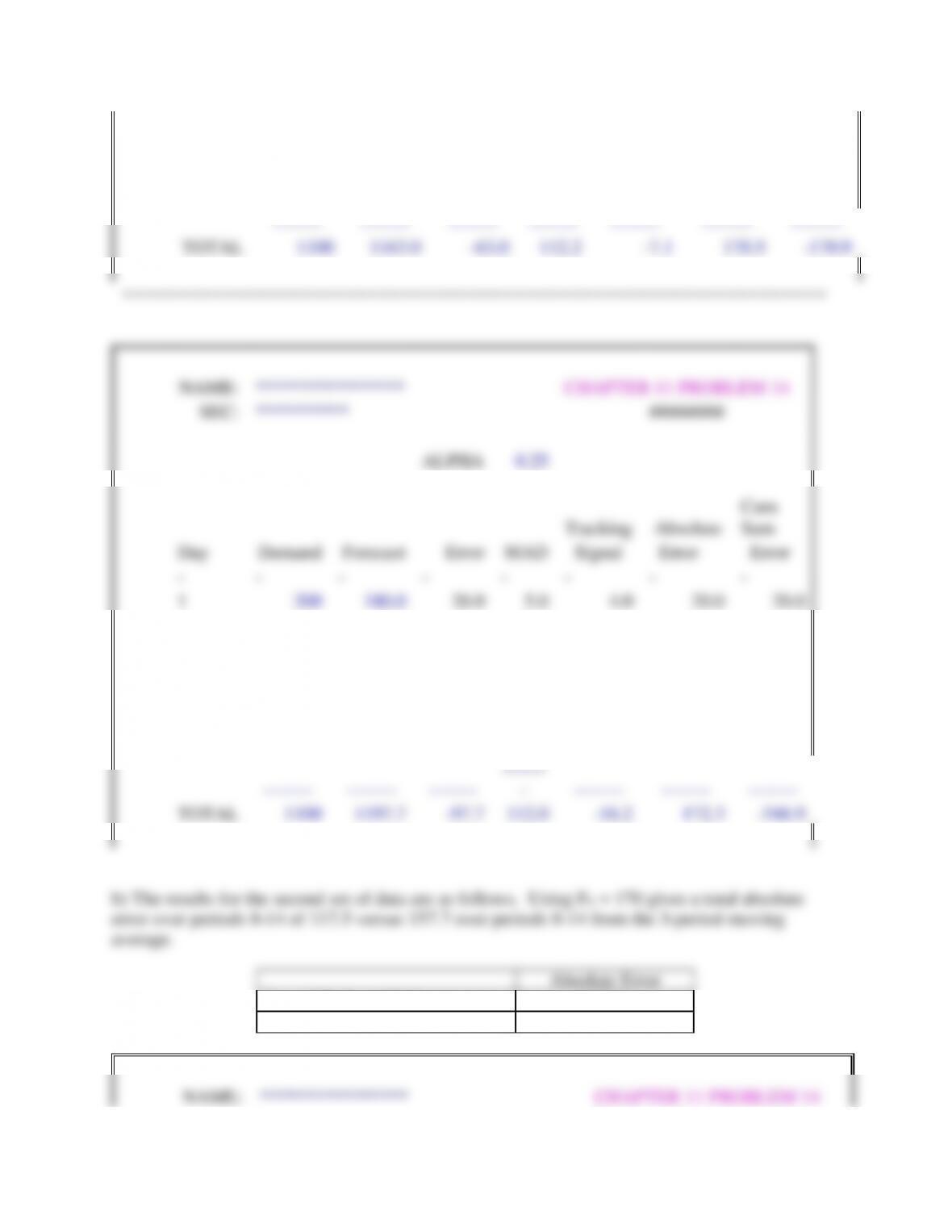
13. a. From the following output for = .2, = .3, and = .4, we see that the smallest
absolute deviation we have at = .2 and = .3, so we look at the bias for these two
values of and we conclude that = .2 gives a model with less bias than = .3.
Thus our final choice is = .2.
Alpha
Absolute Error
Cumulative error
0.2
64.6
-3.6
0.3
64.6
-4.0
0.4
65.3
-3.4

ALPHA
0.2
Tracking
Absolute
Cum Sum
Day
Demand
Forecast
Error
MAD
Signal
Error
Error
–
–
–
–
–
–
–
–
1
200
198.0
2.0
0.4
5.0
2.0
2.0
2
209
198.4
10.6
2.4
5.2
10.6
12.6
3
215
200.5
14.5
4.8
5.6
14.5
27.1
4
180
203.4
-23.4
8.6
0.4
23.4
3.7
5
190
198.7
-8.7
8.6
-0.6
8.7
-5.1
6
195
197.0
-2.0
7.3
-1.0
2.0
-7.1
7
200
196.6
3.4
6.5
-0.6
3.4
-3.6
———
———
———
———
———-
———-
———
TOTALS
1389.0
1392.6
-3.6
38.6
14.1
64.6
ALPHA
0.3
Tracking
Absolute
Cum Sum
Day
Demand
Forecast
Error
MAD
Signal
Error
Error
–
–
–
–
–
–
–
–
1
200
198.0
2.0
0.6
3.3
2.0
2.0
2
209
198.6
10.4
3.5
3.5
10.4
12.4
3
215
201.7
13.3
6.5
4.0
13.3
25.7
4
180
205.7
-25.7
12.2
0.0
25.7
0.0
5
190
198.0
-8.0
11.0
-0.7
8.0
-8.0
6
195
195.6
-0.6
7.9
-1.1
0.6
-8.6
7
200
195.4
4.6
6.9
-0.6
4.6
-4.0
———
———
———
———
———-
———-
———
TOTALS
1389.0
1393.0
-4.0
48.5
8.4
64.6
ALPHA
0.4
Tracking
Absolute
Cum Sum
Day
Demand
Forecast
Error
MAD
Signal
Error
Error
–
–
–
–
–
–
–
–
1
200
198.0
2.0
0.8
2.5
2.0
2.0
2
209
198.8
10.2
4.6
2.7
10.2
12.2
3
215
202.9
12.1
7.6
3.2
12.1
24.3

4
180
207.7
-27.7
15.6
-0.2
27.7
-3.4
5
190
196.6
-6.6
12.0
-0.8
6.6
-10.0
6
195
194.0
1.0
7.6
-1.2
1.0
-9.0
7
200
194.4
5.6
6.8
-0.5
5.6
-3.4
———
———
———
———
———-
———-
———
TOTALS
1389.0
1392.4
-3.4
55.1
5.6
65.3
b. Using the same spreadsheet we calculate the errors for the second set of data.
The smallest error occurs in the model for which = .2. The results are as follows:
Alpha
Absolute Error
Cumulative error
0.2
43.1
-17.9
0.3
43.7
-14.2
0.4
44.2
-11.1
NAME:
****************
CHAPTER 11 PROBLEM 13 B
SEC:
**********
4-Nov-08
ALPHA
0.2
Tracking
Absolute
Cum Sum
Day
Demand
Forecast
Error
MAD
Signal
Error
Error
–
–
–
–
–
–
–
–
8
208
198.0
10.0
2.0
5.0
10.0
10.0
9
186
200.0
-14.0
4.4
-0.9
14.0
-4.0
10
193
197.2
-4.2
4.4
-1.9
4.2
-8.2
11
197
196.4
0.6
3.6
-2.1
0.6
-7.6
12
188
196.5
-8.5
4.6
-3.5
8.5
-16.0
13
191
194.8
-3.8
4.4
-4.5
3.8
-19.8
14
196
194.0
2.0
3.9
-4.5
2.0
-17.9
———
———
———
———
———-
———-
———
TOTALS
1359.0
1376.9
-17.9
27.3
-12.4
43.1
NAME:
****************
CHAPTER 11 PROBLEM 13 B
SEC:
**********
4-Nov-08
ALPHA
0.3
Tracking
Absolute
Cum Sum

Day
Demand
Forecast
Error
MAD
Signal
Error
Error
–
–
–
–
–
–
–
–
8
208
198.0
10.0
3.0
3.3
10.0
10.0
9
186
201.0
-15.0
6.9
-0.7
15.0
-5.0
10
193
196.5
-3.5
6.6
-1.3
3.5
-8.5
11
197
195.5
1.6
5.7
-1.2
1.6
-6.9
12
188
195.9
-7.9
7.0
-2.1
7.9
-14.9
13
191
193.5
-2.5
6.3
-2.8
2.5
-17.4
14
196
192.8
3.2
6.0
-2.4
3.2
-14.2
———
———
———
———
———-
———-
———
TOTALS
1359.0
1373.2
-14.2
41.5
-7.1
43.7
NAME:
****************
CHAPTER 11 PROBLEM 13 B
SEC:
**********
4-Nov-08
ALPHA
0.4
Tracking
Absolute
Cum Sum
Day
Demand
Forecast
Error
MAD
Signal
Error
Error
–
–
–
–
–
–
–
–
8
208
198.0
10.0
4.0
2.5
10.0
10.0
9
186
202.0
-16.0
9.6
-0.6
16.0
-6.0
10
193
195.6
-2.6
8.7
-1.0
2.6
-8.6
11
197
194.6
2.4
8.0
-0.8
2.4
-6.2
12
188
195.5
-7.5
9.4
-1.5
7.5
-13.7
13
191
192.5
-1.5
8.1
-1.9
1.5
-15.2
14
196
191.9
4.1
8.1
-1.4
4.1
-11.1
———
———
———
———
———-
———-
———
TOTALS
1359.0
1370.1
-11.1
55.9
-4.6
44.2
c. This problem illustrates that it is not always straightforward to find the best value for
. By splitting the data into two sets and comparing the forecast errors in both cases, we
14. a. The model that uses F1 = 170 provides the smallest absolute error, based on the
analysis of the historical demand for the first seven days only. The starting forecast value
of 170 is then used to answer part b as shown below.
F1
Absolute Error
160
170.6
170
170.5
180
172.3
NAME:
****************
CHAPTER 11 PROBLEM 14
SEC:
**********
########
ALPHA
0.25
Tracking
Absolute
Cum
Sum
Day
Demand
Forecast
Error
MAD
Signal
Error
Error
–
–
–
–
–
–
–
–
1
200
160.0
40.0
10.0
4.0
40.0
40.0
2
134
170.0
-36.0
16.5
0.2
36.0
4.0
3
147
161.0
-14.0
15.9
-0.6
14.0
-10.0
4
165
157.5
7.5
13.8
-0.2
7.5
-2.5
5
183
159.4
23.6
16.2
1.3
23.6
21.1
6
125
165.3
-40.3
22.3
-0.9
40.3
-19.2
7
146
155.2
-9.2
19.0
-1.5
9.2
-28.4
——–
——–
——–
—-—
–
——–
——–
——–
TOTAL
1100
1128.4
-28.4
113.6
2.4
170.6
5.1
================================================================
NAME:
****************
CHAPTER 11 PROBLEM 14
SEC:
**********
########
ALPHA
0.25
Tracking
Absolute
Cum
Sum
Day
Demand
Forecast
Error
MAD
Signal
Error
Error
–
–
–
–
–
–
–
–
1
200
170.0
30.0
7.5
4.0
30.0
30.0
2
134
177.5
-43.5
16.5
-0.8
43.5
-13.5
3
147
166.6
-19.6
17.3
-1.9
19.6
-33.1
4
165
161.7
3.3
13.8
-2.2
3.3
-29.8
5
183
162.5
20.5
15.5
-0.6
20.5
-9.4
6
125
167.7
-42.7
22.3
-2.3
42.7
-52.0
7
146
157.0
-11.0
19.4
-3.2
11.0
-63.0
——–
——–
——–
——–
——–
——–
——–
TOTAL
1100
1163.0
-63.0
112.2
-7.1
170.5
-170.9
===============================================================
NAME:
****************
CHAPTER 11 PROBLEM 14
SEC:
**********
########
ALPHA
0.25
Tracking
Absolute
Cum
Sum
Day
Demand
Forecast
Error
MAD
Signal
Error
Error
–
–
–
–
–
–
–
–
1
200
180.0
20.0
5.0
4.0
20.0
20.0
2
134
185.0
-51.0
16.5
-1.9
51.0
-31.0
3
147
172.3
-25.3
18.7
-3.0
25.3
-56.3
4
165
165.9
-0.9
14.3
-4.0
0.9
-57.2
5
183
165.7
17.3
15.0
-2.7
17.3
-39.9
6
125
170.0
-45.0
22.5
-3.8
45.0
-84.9
7
146
158.8
-12.8
20.1
-4.9
12.8
-97.7
——–
——–
——–
—-—
–
——–
——–
——–
TOTAL
1100
1197.7
-97.7
112.0
-16.2
172.3
-346.9
3-period Moving Average
3-period Moving Average
ALPHA
0.2
Tracking
Absolute
Cum Sum
Day
Demand
Forecast
Error
MAD
Signal
Error
Error
–
–
–
–
–
–
–
–
1
200
198.0
2.0
0.4
5.0
2.0
2.0
2
209
198.4
10.6
2.4
5.2
10.6
12.6
3
215
200.5
14.5
4.8
5.6
14.5
27.1
4
180
203.4
-23.4
8.6
0.4
23.4
3.7
5
190
198.7
-8.7
8.6
-0.6
8.7
-5.1
6
195
197.0
-2.0
7.3
-1.0
2.0
-7.1
7
200
196.6
3.4
6.5
-0.6
3.4
-3.6
———
———
———
———
———-
———-
———
TOTALS
1389.0
1392.6
-3.6
38.6
14.1
64.6
ALPHA
0.3
Tracking
Absolute
Cum Sum
Day
Demand
Forecast
Error
MAD
Signal
Error
Error
–
–
–
–
–
–
–
–
1
200
198.0
2.0
0.6
3.3
2.0
2.0
2
209
198.6
10.4
3.5
3.5
10.4
12.4
3
215
201.7
13.3
6.5
4.0
13.3
25.7
4
180
205.7
-25.7
12.2
0.0
25.7
0.0
5
190
198.0
-8.0
11.0
-0.7
8.0
-8.0
6
195
195.6
-0.6
7.9
-1.1
0.6
-8.6
7
200
195.4
4.6
6.9
-0.6
4.6
-4.0
———
———
———
———
———-
———-
———
TOTALS
1389.0
1393.0
-4.0
48.5
8.4
64.6
ALPHA
0.4
Tracking
Absolute
Cum Sum
Day
Demand
Forecast
Error
MAD
Signal
Error
Error
–
–
–
–
–
–
–
–
1
200
198.0
2.0
0.8
2.5
2.0
2.0
2
209
198.8
10.2
4.6
2.7
10.2
12.2
3
215
202.9
12.1
7.6
3.2
12.1
24.3
4
180
207.7
-27.7
15.6
-0.2
27.7
-3.4
5
190
196.6
-6.6
12.0
-0.8
6.6
-10.0
6
195
194.0
1.0
7.6
-1.2
1.0
-9.0
7
200
194.4
5.6
6.8
-0.5
5.6
-3.4
———
———
———
———
———-
———-
———
TOTALS
1389.0
1392.4
-3.4
55.1
5.6
65.3
b. Using the same spreadsheet we calculate the errors for the second set of data.
The smallest error occurs in the model for which = .2. The results are as follows:
Alpha
Absolute Error
Cumulative error
0.2
43.1
-17.9
0.3
43.7
-14.2
0.4
44.2
-11.1
NAME:
****************
CHAPTER 11 PROBLEM 13 B
SEC:
**********
4-Nov-08
ALPHA
0.2
Tracking
Absolute
Cum Sum
Day
Demand
Forecast
Error
MAD
Signal
Error
Error
–
–
–
–
–
–
–
–
8
208
198.0
10.0
2.0
5.0
10.0
10.0
9
186
200.0
-14.0
4.4
-0.9
14.0
-4.0
10
193
197.2
-4.2
4.4
-1.9
4.2
-8.2
11
197
196.4
0.6
3.6
-2.1
0.6
-7.6
12
188
196.5
-8.5
4.6
-3.5
8.5
-16.0
13
191
194.8
-3.8
4.4
-4.5
3.8
-19.8
14
196
194.0
2.0
3.9
-4.5
2.0
-17.9
———
———
———
———
———-
———-
———
TOTALS
1359.0
1376.9
-17.9
27.3
-12.4
43.1
NAME:
****************
CHAPTER 11 PROBLEM 13 B
SEC:
**********
4-Nov-08
ALPHA
0.3
Tracking
Absolute
Cum Sum
Day
Demand
Forecast
Error
MAD
Signal
Error
Error
–
–
–
–
–
–
–
–
8
208
198.0
10.0
3.0
3.3
10.0
10.0
9
186
201.0
-15.0
6.9
-0.7
15.0
-5.0
10
193
196.5
-3.5
6.6
-1.3
3.5
-8.5
11
197
195.5
1.6
5.7
-1.2
1.6
-6.9
12
188
195.9
-7.9
7.0
-2.1
7.9
-14.9
13
191
193.5
-2.5
6.3
-2.8
2.5
-17.4
14
196
192.8
3.2
6.0
-2.4
3.2
-14.2
———
———
———
———
———-
———-
———
TOTALS
1359.0
1373.2
-14.2
41.5
-7.1
43.7
NAME:
****************
CHAPTER 11 PROBLEM 13 B
SEC:
**********
4-Nov-08
ALPHA
0.4
Tracking
Absolute
Cum Sum
Day
Demand
Forecast
Error
MAD
Signal
Error
Error
–
–
–
–
–
–
–
–
8
208
198.0
10.0
4.0
2.5
10.0
10.0
9
186
202.0
-16.0
9.6
-0.6
16.0
-6.0
10
193
195.6
-2.6
8.7
-1.0
2.6
-8.6
11
197
194.6
2.4
8.0
-0.8
2.4
-6.2
12
188
195.5
-7.5
9.4
-1.5
7.5
-13.7
13
191
192.5
-1.5
8.1
-1.9
1.5
-15.2
14
196
191.9
4.1
8.1
-1.4
4.1
-11.1
———
———
———
———
———-
———-
———
TOTALS
1359.0
1370.1
-11.1
55.9
-4.6
44.2
c. This problem illustrates that it is not always straightforward to find the best value for
. By splitting the data into two sets and comparing the forecast errors in both cases, we
14. a. The model that uses F1 = 170 provides the smallest absolute error, based on the
analysis of the historical demand for the first seven days only. The starting forecast value
of 170 is then used to answer part b as shown below.
F1
Absolute Error
160
170.6
170
170.5
180
172.3
NAME:
****************
CHAPTER 11 PROBLEM 14
SEC:
**********
########
ALPHA
0.25
Tracking
Absolute
Cum
Sum
Day
Demand
Forecast
Error
MAD
Signal
Error
Error
–
–
–
–
–
–
–
–
1
200
160.0
40.0
10.0
4.0
40.0
40.0
2
134
170.0
-36.0
16.5
0.2
36.0
4.0
3
147
161.0
-14.0
15.9
-0.6
14.0
-10.0
4
165
157.5
7.5
13.8
-0.2
7.5
-2.5
5
183
159.4
23.6
16.2
1.3
23.6
21.1
6
125
165.3
-40.3
22.3
-0.9
40.3
-19.2
7
146
155.2
-9.2
19.0
-1.5
9.2
-28.4
——–
——–
——–
—-—
–
——–
——–
——–
TOTAL
1100
1128.4
-28.4
113.6
2.4
170.6
5.1
================================================================
NAME:
****************
CHAPTER 11 PROBLEM 14
SEC:
**********
########
ALPHA
0.25
Tracking
Absolute
Cum
Sum
Day
Demand
Forecast
Error
MAD
Signal
Error
Error
–
–
–
–
–
–
–
–
1
200
170.0
30.0
7.5
4.0
30.0
30.0
2
134
177.5
-43.5
16.5
-0.8
43.5
-13.5
3
147
166.6
-19.6
17.3
-1.9
19.6
-33.1
4
165
161.7
3.3
13.8
-2.2
3.3
-29.8
5
183
162.5
20.5
15.5
-0.6
20.5
-9.4
6
125
167.7
-42.7
22.3
-2.3
42.7
-52.0
7
146
157.0
-11.0
19.4
-3.2
11.0
-63.0
——–
——–
——–
——–
——–
——–
——–
TOTAL
1100
1163.0
-63.0
112.2
-7.1
170.5
-170.9
===============================================================
NAME:
****************
CHAPTER 11 PROBLEM 14
SEC:
**********
########
ALPHA
0.25
Tracking
Absolute
Cum
Sum
Day
Demand
Forecast
Error
MAD
Signal
Error
Error
–
–
–
–
–
–
–
–
1
200
180.0
20.0
5.0
4.0
20.0
20.0
2
134
185.0
-51.0
16.5
-1.9
51.0
-31.0
3
147
172.3
-25.3
18.7
-3.0
25.3
-56.3
4
165
165.9
-0.9
14.3
-4.0
0.9
-57.2
5
183
165.7
17.3
15.0
-2.7
17.3
-39.9
6
125
170.0
-45.0
22.5
-3.8
45.0
-84.9
7
146
158.8
-12.8
20.1
-4.9
12.8
-97.7
——–
——–
——–
—-—
–
——–
——–
——–
TOTAL
1100
1197.7
-97.7
112.0
-16.2
172.3
-346.9