
Chapter 11
Forecasting
Teaching Notes
The reference list includes some recommended books and articles on forecasting. The

4. Qualitative methods may be most appropriate if historical data about past demand are
unavailable or inappropriate due to major changes or expected changes or if the cost of
obtaining historical data is high relative to the expected benefits of an accurate forecast.
5. Qualitative forecasts are useful for long-range time horizons and for such purposes as
process design, capacity planning and facilities location. They are most useful when no
historical data exists or when existing data are not applicable.
Time-series forecasts are primarily useful in the short term for purposes such as materials
management, purchasing, and scheduling.
6. For inventory and scheduling, there are usually a large number of products to consider and
decisions tend to be repetitive and frequent. Generally the cost required to make a
qualitative or causal forecast is large relative to possible improvements in accuracy;
additionally, the time requirements make it difficult to produce forecasts as frequently as
required for inventory and scheduling decisions.
7. a. Monthly sales of a retail florist: Seasonal, trend and random.
b. Monthly sales of milk in a supermarket: Trend and random.
c. Daily demand for telephone calls: Seasonal (day of week and holidays), trend and
random.
8. Exponential smoothing requires less storage of data than the moving average methods.
Only two pieces of data must be stored ( and Ft) for exponential smoothing methods. The
moving average methods require storage of N pieces of data plus the value of N. The
weighted moving average method further requires the storage of the weights.
9. The data should be divided into two parts. The first part should be used to try different
levels of , and those with the lowest bias and variance should be selected. These ‘s
should then be tested on the second part of the data and the best selected for use.
10. Fit refers to how well a proposed model explains the data points used to determine that
model; i.e., some measure of explained variance. Prediction refers to how well that model
predicts new points; i.e., the degree of forecast error.
11. At the aggregate level we can expect some bias. If the forecasts are used for control
purposes, they will probably tend to be understated; if not, the forecasts are likely to be

overly optimistic. If the bias is known, it may be possible to adjust the aggregated forecasts
to compensate for the bias.
At the level of specific inventory and scheduling decisions, this method is likely to result
12. The solution to this situation is to get marketing and operations together to discuss the
forecasts. First, the purpose of the marketing and operations forecasts should be discussed
to see if this leads to the different forecasts. Perhaps, marketing is using their forecast as a
sales target or goal rather than a production requirement. If the goals are similar, then the
methods of forecasting might be leading to the differences. In this case marketing and
operations can discuss the forecasting accuracy of each method and jointly define a method
13. The purpose of CPFR is to achieve more accurate forecasts. This is done by customers and
suppliers in the supply chain collaborating on planning and forecasting. If the forecasts of
the supplier and customer do not agree, collaboration is used to arrive at a mutually
acceptable forecast and replenishment plan. The supplier benefits by learning of changes
in advertising or special promotions that the customer is planning, adjustments in the
customer’s inventory or possible demand shifts. The customers benefit in having the
14. CPFR is useful when there are a relatively small number of suppliers that provide most of
the product purchased by the customer (80-20 rule). If there were too many suppliers, it
would be very expensive for the customer to collaborate with each supplier. On the other
hand, a supplier would not use CPFR if there were too many customers. This is true in
many retail situations such as grocery stores and big box stores in which there are thousands
of customers. On the other hand, most retailers only have a handful of significant suppliers

1. Period Demand At(3period) At (5period)
1 85 – –
2 92 – –
3 71 82.7 –
4 97 86.7 –
5 93 87.0 87.6
6 82 90.7 87.0
7 89 88.0 86.4
2. a. At Ft
Dt 3 – Period 3 – Period Dt – Ft
October Demand Moving Average Forecast Error
1 92
2 127
3 106 108.3
4 165 132.7 108.3 56.7
5 125 132.0 132.7 -7.7
6 111 133.7 132.0 -21.0
7 178 138.0 133.7 44.3
8 97 128.7 138.0 –41.0
2 b.
Weighted Dt – Ft
October Dt At Ft Error
1 92
2 127
3 106 109.5
4 165 139.7 109.5 55.5
5 125 133.2 139.7 -14.7
6 111 126.0 133.2 -22.2
7 178 147.3 126.0 52.0
8 97 124.1 147.3 -50.3
(Weightings: W1 = .5 W2 = .3 W3 = .2)
c. A. Arithmetic sum of errors
3 period moving average 31.3
Weighted average 20.3
B. Absolute deviation
3 period moving average 170.7
Weighted average 194.7
Neither is better. The weighted average has a smaller arithmetic sum of errors, but the 3
period moving average has smaller absolute deviation.
3. a.
Day
Dt
Demand
At
3-Period
Mov.Avg.
Ft
3-Period
Forecast
Dt-Ft
Error
At
5-Period
Mov.Avg.
Ft
5-Period
Forecast
Dt-Ft
Error
1
200
2
134
3
147
160.33
4
165
148.67
160.33
4.67
5
183
165.00
148.67
34.33
165.80
6
125
157.67
165.00
-40.00
150.80
165.80
-40.80
7
146
151.33
157.67
-11.67
153.20
150.80
-4.80
8
154
141.67
151.33
2.67
154.60
153.20
0.80
9
182
160.67
141.67
40.33
158.00
154.60
27.40
10
197
177.67
160.67
36.33
160.80
158.00
39.00
11
132
170.33
177.67
-45.67
162.20
160.80
-28.80
12
163
164.00
170.33
-7.33
165.60
162.20
0.80
13
157
150.67
164.00
-7.00
166.20
165.60
-8.60
14
169
163.00
150.67
18.33
163.60
166.20
2.80
c. The 5-period moving average is better because it smoothes the wide demand swings.
3-Period Moving Average 2.27
5-Period Moving Average -1.36
Average Absolute Deviation
3-Period Moving Average 22.58
5-Period Moving Average 17.09
4. a. F t+1 = F t + (D t – F t)
F t+1 = 110,000 + .1 (130,000 – 110,000)
F t+1 = 112,000
5. a. Ft+1 = F t + (D t – F t)
F t+1 = 100,000 + .1 (90,000 – 100,000)
F t+1 = 99,000
6. = .1 = .3
Period Dt Ft Dt – Ft Ft Dt – Ft
1
92
90
2
90
2
2
127
90.2
36.8
90.6
36.4
3
106
93.9
12.1
101.5
4.5

4
165
95.1
69.9
102.9
62.1
5
125
102.1
22.9
121.5
3.5
6
111
104.4
6.6
122.6
-11.6
7
178
105.0
73.0
119.1
58.9
8
97
112.3
-15.3
136.8
-39.8
110.8
124.8
7. Refer to problem # 6.
Arithmetic Sum (Bias Error) = .1 = .3
(Dt – Ft) = 208.0 116.8
Absolute Deviation
8. a.
NAME:
****************
CHAPTER 11 PROBLEM 8
SEC:
**********
6-Aug-
07
ALPHA
0.1
Tracking
Absolute
CumSum
Day
Demand
Forecast
Error
MAD
Signal
Error
Error
1
200
100.0
100.0
10.0
10.0
100.0
100.0
2
134
110.0
24.0
11.4
10.9
24.0
124.0
3
147
112.4
34.6
13.7
11.6
34.6
158.6
4
165
115.9
49.1
17.3
12.0
49.1
207.7
5
183
120.8
62.2
21.8
12.4
62.2
270.0
6
125
127.0
-2.0
19.8
13.5
2.0
268.0
7
146
126.8
19.2
19.7
14.6
19.2
287.2
8
154
128.7
25.3
20.3
15.4
25.3
312.5
9
182
131.2
50.8
23.3
15.6
50.8
363.2
10
197
136.3
60.7
27.1
15.7
60.7
423.9
11
132
142.4
-10.4
25.4
16.3
10.4
413.5
12
163
141.3
21.7
25.0
17.4
21.7
435.1
13
157
143.5
13.5
23.9
18.8
13.5
448.6
14
169
144.9
24.1
23.9
19.8
24.1
472.8
——–
——–
——-
——-
———
———
——–
TOTALS
2254.0
1781.2
472.8
282.5
203.9
497.5
8. a. (continued) Henry’s = .3 produces better results according to the cumulative sum of the
error and cumulative sum of the absolute error. However, the tracking signal is too large
on both of these forecasts, exceeding ±6. Neither forecast is, therefore, very good because
the starting forecast is too low; F1 = 200, for example, would produce a much better
forecast.
8. b.
ALPHA
Tracking
Absolute
Day
1
100.0
100.0
2
3
4
5
6
7
8
9
10
11
12
13
14
——–
——-
——
———
———
——–
TOTALS
2254.0
2047.0
207.0
319.6
109.9
353.4
ALPHA
Tracking
Absolute
Day
1
100.0
100.0
2
3
4
5
6
7
8
9
10
11
12
13
14
——–
——-
——
———
———
——–
TOTALS
2254.0
2047.0
207.0
319.6
109.9
353.4
8. c. Increasing the value of alpha would generally decrease forecasts error. However,
without changing the F1 from 100 to a greater value (closer to 200) will simply bias
future forecasts to the low side.
Error Absolute Error Period 14
Cumulative sum Cumulative sum Tracking signal
9.
Period
Dt
Ft
et
MADt
Tracking
Signal
0
20
1
300
290
10
19
.526
2
280
291
-11
18.2
-.055
3
309
289.9
19.1
18.3
.989
10.
Period
Dt
At
Ft
et
MADt
Tracking Signal
0
16.00
1
1
20
17.60
16.00
4.00
2.20
1.82
2
26
20.96
17.60
8.40
4.68
2.65
3
14
18.18
20.96
-6.96
5.59
0.97
11. a. and b.
0
50
100
150
200
250
Demand and Forecasts 11-8b
Demand
α = .1 Forecasts
α = .3 Forecasts
NAME:
**************
CHAPTER 11, PROBLEM 11
SECTION:
**********
04 Apr 2010
ALPHA =
0.2
TRACKING
DEMAND
FORECAST
ERROR
MAD
SIGNAL
MONDAY
80
85.00
-5.00
1.00
-5.00
TUESDAY
53
84.00
-31.00
7.00
-5.14
WEDNESDAY
65
77.80
-12.80
8.16
-5.98
THURSDAY
43
75.24
-32.24
12.98
-6.25
FRIDAY
85
68.79
16.21
13.62
-4.76
SATURDAY
101
72.03
28.97
16.69
-2.15
TOTALS
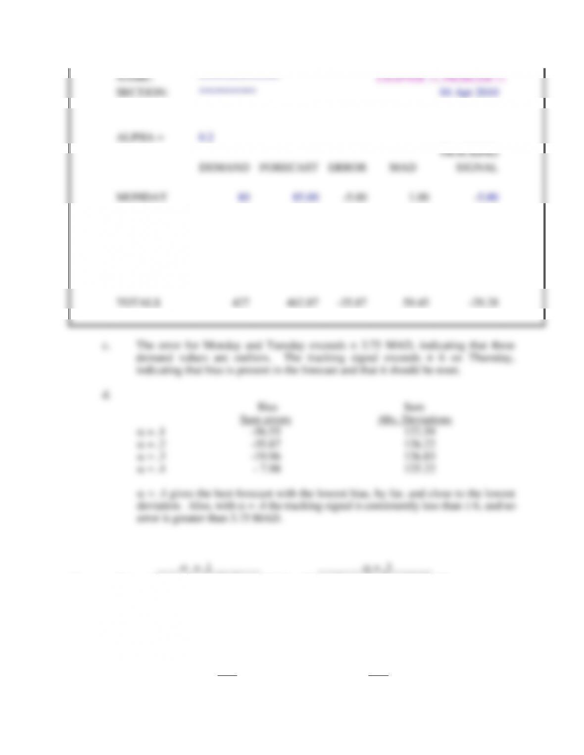
427
462.87
-35.87
59.45
-29.28
12. a. Day Dt Ft et MAD TS Ft et MAD TS
1 35 33.0 2.0 0.2 10.0 33.0 2.0 0.6 3.3
2 47 33.2 13.8 1.6 10.1 33.6 13.4 4.4 3.5
3 46 34.6 11.4 2.5 10.7 37.6 8.4 5.6 4.2
4 39 35.7 3.3 2.6 11.6 40.1 1.1 4.3 5.3
5 26 36.0 10.0 3.4 6.1 39.8 13.8 7.1 1.2
6 33 35.0 2.0 3.2 5.7 35.7 2.7 5.8 1.1
7 24 34.8 10.8 4.0 1.9 34.9 10.9 7.3 -0.6
4. Qualitative methods may be most appropriate if historical data about past demand are
unavailable or inappropriate due to major changes or expected changes or if the cost of
obtaining historical data is high relative to the expected benefits of an accurate forecast.
5. Qualitative forecasts are useful for long-range time horizons and for such purposes as
process design, capacity planning and facilities location. They are most useful when no
historical data exists or when existing data are not applicable.
Time-series forecasts are primarily useful in the short term for purposes such as materials
management, purchasing, and scheduling.
6. For inventory and scheduling, there are usually a large number of products to consider and
decisions tend to be repetitive and frequent. Generally the cost required to make a
qualitative or causal forecast is large relative to possible improvements in accuracy;
additionally, the time requirements make it difficult to produce forecasts as frequently as
required for inventory and scheduling decisions.
7. a. Monthly sales of a retail florist: Seasonal, trend and random.
b. Monthly sales of milk in a supermarket: Trend and random.
c. Daily demand for telephone calls: Seasonal (day of week and holidays), trend and
random.
8. Exponential smoothing requires less storage of data than the moving average methods.
Only two pieces of data must be stored ( and Ft) for exponential smoothing methods. The
moving average methods require storage of N pieces of data plus the value of N. The
weighted moving average method further requires the storage of the weights.
9. The data should be divided into two parts. The first part should be used to try different
levels of , and those with the lowest bias and variance should be selected. These ‘s
should then be tested on the second part of the data and the best selected for use.
10. Fit refers to how well a proposed model explains the data points used to determine that
model; i.e., some measure of explained variance. Prediction refers to how well that model
predicts new points; i.e., the degree of forecast error.
11. At the aggregate level we can expect some bias. If the forecasts are used for control
purposes, they will probably tend to be understated; if not, the forecasts are likely to be
overly optimistic. If the bias is known, it may be possible to adjust the aggregated forecasts
to compensate for the bias.
At the level of specific inventory and scheduling decisions, this method is likely to result
12. The solution to this situation is to get marketing and operations together to discuss the
forecasts. First, the purpose of the marketing and operations forecasts should be discussed
to see if this leads to the different forecasts. Perhaps, marketing is using their forecast as a
sales target or goal rather than a production requirement. If the goals are similar, then the
methods of forecasting might be leading to the differences. In this case marketing and
operations can discuss the forecasting accuracy of each method and jointly define a method
13. The purpose of CPFR is to achieve more accurate forecasts. This is done by customers and
suppliers in the supply chain collaborating on planning and forecasting. If the forecasts of
the supplier and customer do not agree, collaboration is used to arrive at a mutually
acceptable forecast and replenishment plan. The supplier benefits by learning of changes
in advertising or special promotions that the customer is planning, adjustments in the
customer’s inventory or possible demand shifts. The customers benefit in having the
14. CPFR is useful when there are a relatively small number of suppliers that provide most of
the product purchased by the customer (80-20 rule). If there were too many suppliers, it
would be very expensive for the customer to collaborate with each supplier. On the other
hand, a supplier would not use CPFR if there were too many customers. This is true in
many retail situations such as grocery stores and big box stores in which there are thousands
of customers. On the other hand, most retailers only have a handful of significant suppliers
1. Period Demand At(3period) At (5period)
1 85 – –
2 92 – –
3 71 82.7 –
4 97 86.7 –
5 93 87.0 87.6
6 82 90.7 87.0
7 89 88.0 86.4
2. a. At Ft
Dt 3 – Period 3 – Period Dt – Ft
October Demand Moving Average Forecast Error
1 92
2 127
3 106 108.3
4 165 132.7 108.3 56.7
5 125 132.0 132.7 -7.7
6 111 133.7 132.0 -21.0
7 178 138.0 133.7 44.3
8 97 128.7 138.0 –41.0
2 b.
Weighted Dt – Ft
October Dt At Ft Error
1 92
2 127
3 106 109.5
4 165 139.7 109.5 55.5
5 125 133.2 139.7 -14.7
6 111 126.0 133.2 -22.2
7 178 147.3 126.0 52.0
8 97 124.1 147.3 -50.3
(Weightings: W1 = .5 W2 = .3 W3 = .2)
c. A. Arithmetic sum of errors
3 period moving average 31.3
Weighted average 20.3
B. Absolute deviation
3 period moving average 170.7
Weighted average 194.7
Neither is better. The weighted average has a smaller arithmetic sum of errors, but the 3
period moving average has smaller absolute deviation.
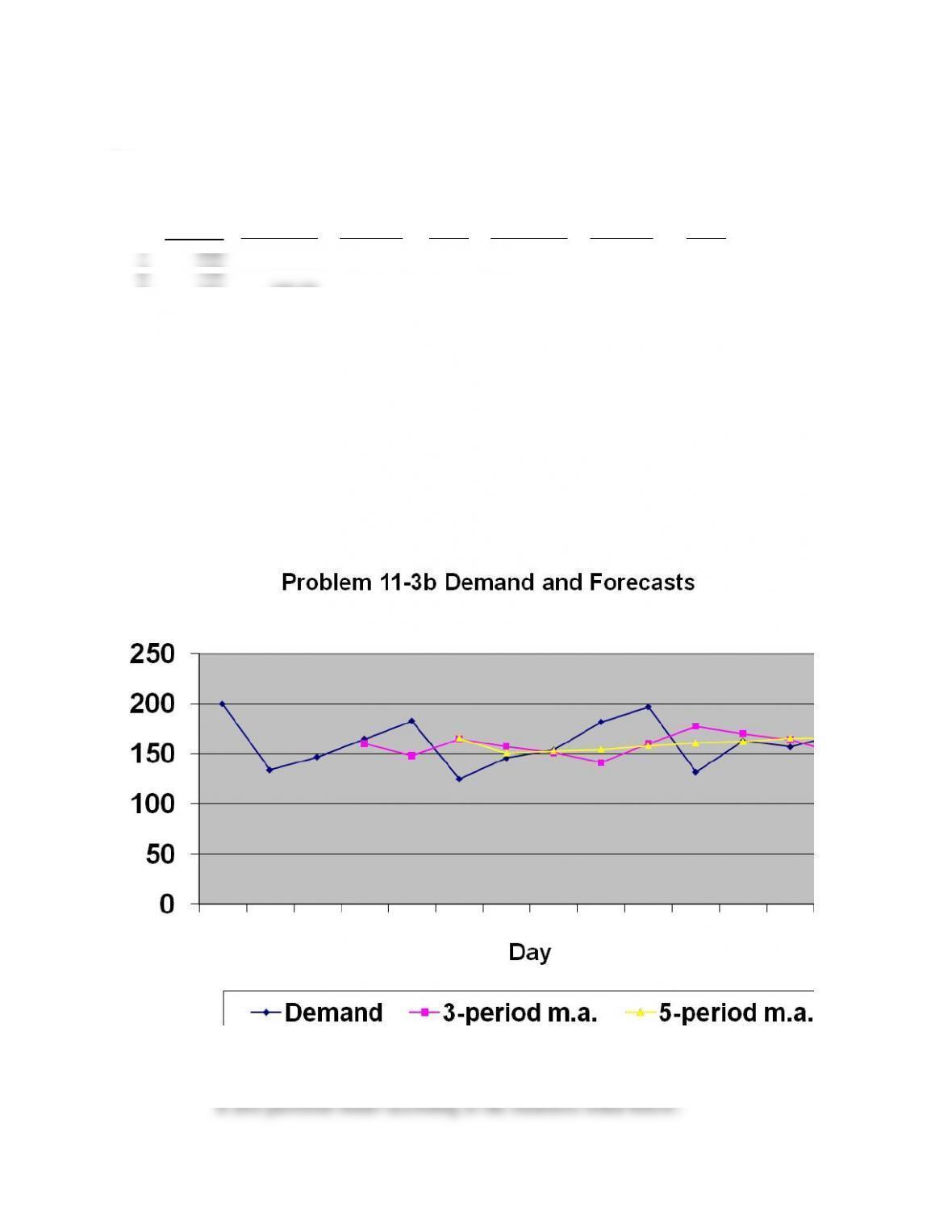
3. a.
Day
Dt
Demand
At
3-Period
Mov.Avg.
Ft
3-Period
Forecast
Dt-Ft
Error
At
5-Period
Mov.Avg.
Ft
5-Period
Forecast
Dt-Ft
Error
1
200
2
134
3
147
160.33
4
165
148.67
160.33
4.67
5
183
165.00
148.67
34.33
165.80
6
125
157.67
165.00
-40.00
150.80
165.80
-40.80
7
146
151.33
157.67
-11.67
153.20
150.80
-4.80
8
154
141.67
151.33
2.67
154.60
153.20
0.80
9
182
160.67
141.67
40.33
158.00
154.60
27.40
10
197
177.67
160.67
36.33
160.80
158.00
39.00
11
132
170.33
177.67
-45.67
162.20
160.80
-28.80
12
163
164.00
170.33
-7.33
165.60
162.20
0.80
13
157
150.67
164.00
-7.00
166.20
165.60
-8.60
14
169
163.00
150.67
18.33
163.60
166.20
2.80
c. The 5-period moving average is better because it smoothes the wide demand swings.
3-Period Moving Average 2.27
5-Period Moving Average -1.36
Average Absolute Deviation
3-Period Moving Average 22.58
5-Period Moving Average 17.09
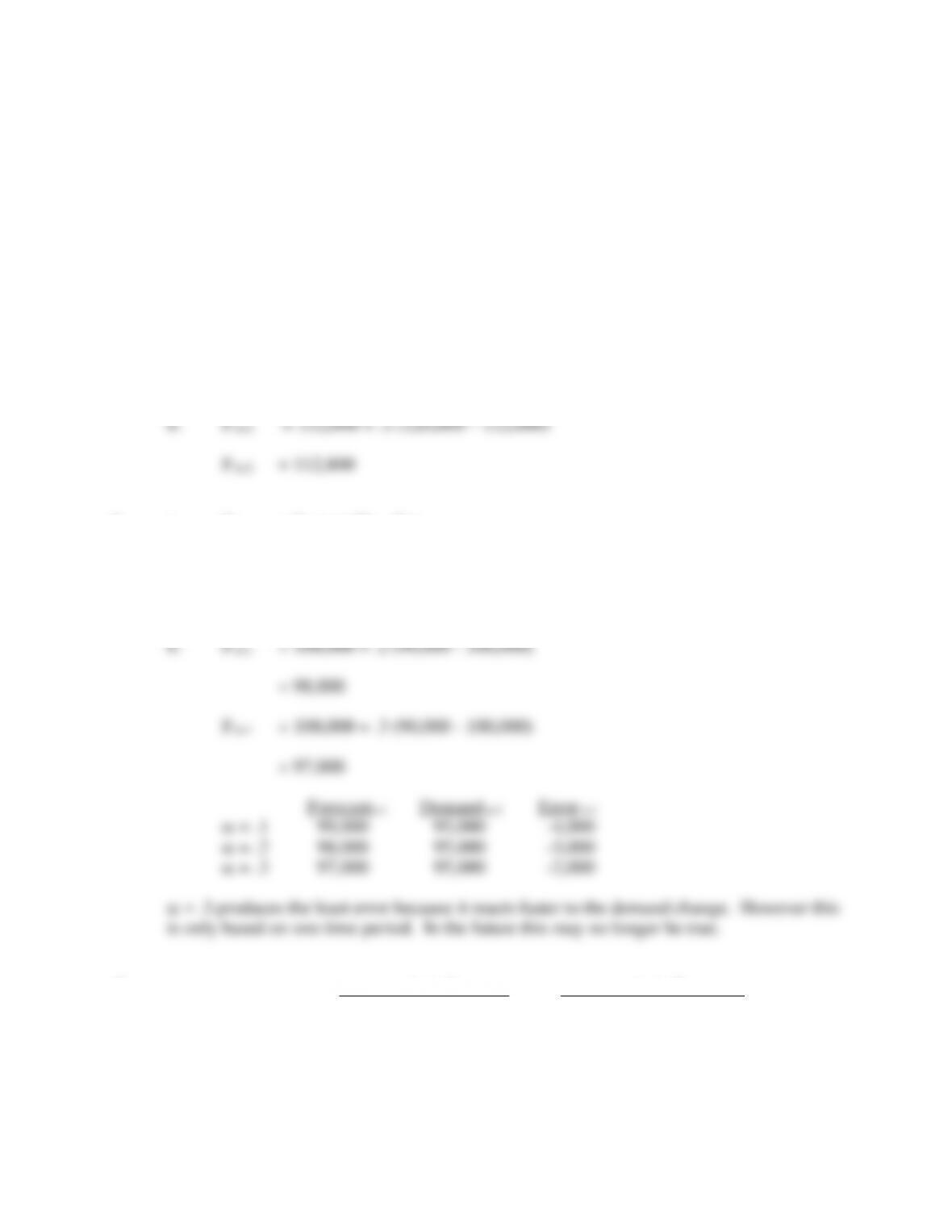
4. a. F t+1 = F t + (D t – F t)
F t+1 = 110,000 + .1 (130,000 – 110,000)
F t+1 = 112,000
5. a. Ft+1 = F t + (D t – F t)
F t+1 = 100,000 + .1 (90,000 – 100,000)
F t+1 = 99,000
6. = .1 = .3
Period Dt Ft Dt – Ft Ft Dt – Ft
1
92
90
2
90
2
2
127
90.2
36.8
90.6
36.4
3
106
93.9
12.1
101.5
4.5
4
165
95.1
69.9
102.9
62.1
5
125
102.1
22.9
121.5
3.5
6
111
104.4
6.6
122.6
-11.6
7
178
105.0
73.0
119.1
58.9
8
97
112.3
-15.3
136.8
-39.8
110.8
124.8
7. Refer to problem # 6.
Arithmetic Sum (Bias Error) = .1 = .3
(Dt – Ft) = 208.0 116.8
Absolute Deviation
8. a.
NAME:
****************
CHAPTER 11 PROBLEM 8
SEC:
**********
6-Aug-
07
ALPHA
0.1
Tracking
Absolute
CumSum
Day
Demand
Forecast
Error
MAD
Signal
Error
Error
1
200
100.0
100.0
10.0
10.0
100.0
100.0
2
134
110.0
24.0
11.4
10.9
24.0
124.0
3
147
112.4
34.6
13.7
11.6
34.6
158.6
4
165
115.9
49.1
17.3
12.0
49.1
207.7
5
183
120.8
62.2
21.8
12.4
62.2
270.0
6
125
127.0
-2.0
19.8
13.5
2.0
268.0
7
146
126.8
19.2
19.7
14.6
19.2
287.2
8
154
128.7
25.3
20.3
15.4
25.3
312.5
9
182
131.2
50.8
23.3
15.6
50.8
363.2
10
197
136.3
60.7
27.1
15.7
60.7
423.9
11
132
142.4
-10.4
25.4
16.3
10.4
413.5
12
163
141.3
21.7
25.0
17.4
21.7
435.1
13
157
143.5
13.5
23.9
18.8
13.5
448.6
14
169
144.9
24.1
23.9
19.8
24.1
472.8
——–
——–
——-
——-
———
———
——–
TOTALS
2254.0
1781.2
472.8
282.5
203.9
497.5
8. a. (continued) Henry’s = .3 produces better results according to the cumulative sum of the
error and cumulative sum of the absolute error. However, the tracking signal is too large
on both of these forecasts, exceeding ±6. Neither forecast is, therefore, very good because
the starting forecast is too low; F1 = 200, for example, would produce a much better
forecast.
8. b.
8. c. Increasing the value of alpha would generally decrease forecasts error. However,
without changing the F1 from 100 to a greater value (closer to 200) will simply bias
future forecasts to the low side.
Error Absolute Error Period 14
Cumulative sum Cumulative sum Tracking signal
9.
Period
Dt
Ft
et
MADt
Tracking
Signal
0
20
1
300
290
10
19
.526
2
280
291
-11
18.2
-.055
3
309
289.9
19.1
18.3
.989
10.
Period
Dt
At
Ft
et
MADt
Tracking Signal
0
16.00
1
1
20
17.60
16.00
4.00
2.20
1.82
2
26
20.96
17.60
8.40
4.68
2.65
3
14
18.18
20.96
-6.96
5.59
0.97
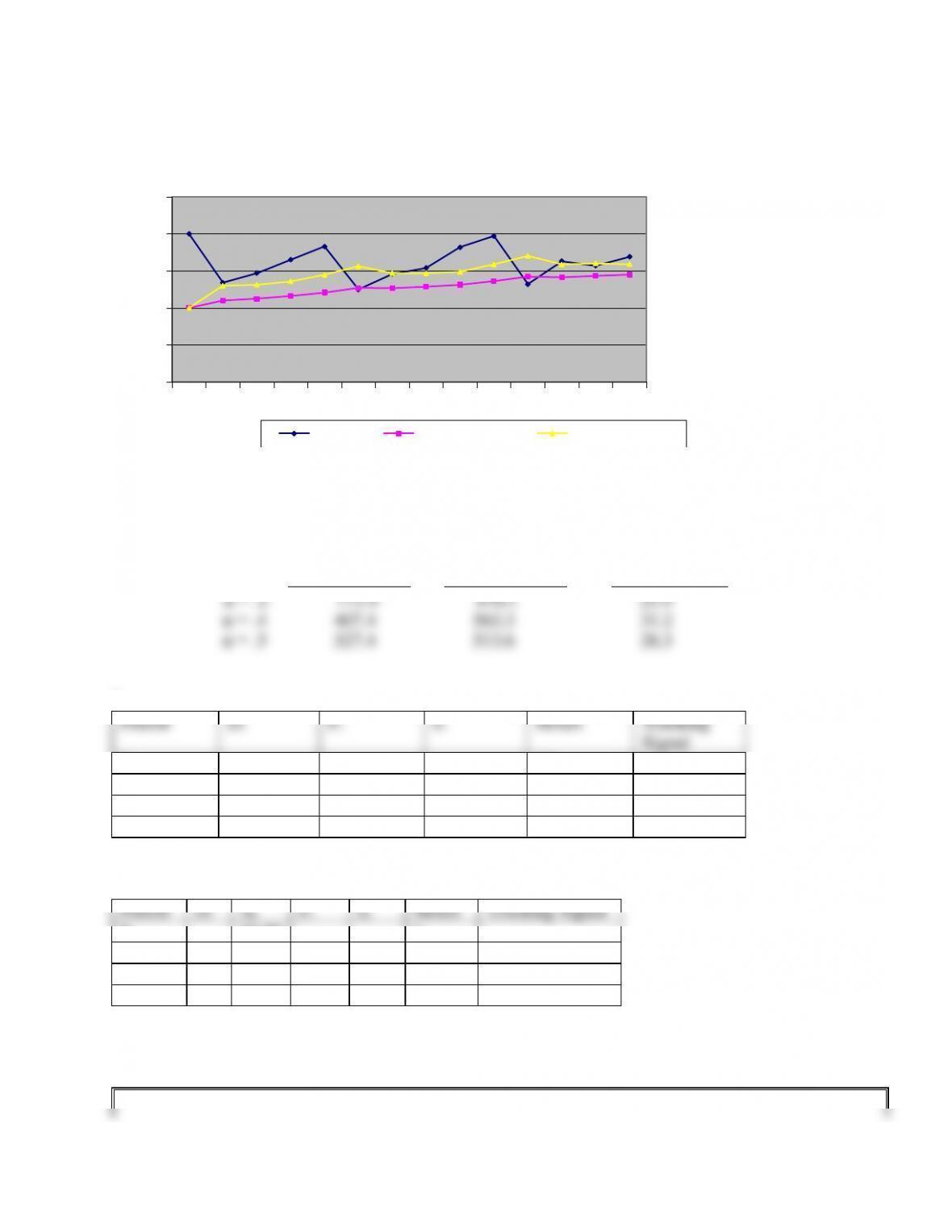
11. a. and b.
0
50
100
150
200
250
Demand and Forecasts 11-8b
Demand
α = .1 Forecasts
α = .3 Forecasts
NAME:
**************
CHAPTER 11, PROBLEM 11
SECTION:
**********
04 Apr 2010
ALPHA =
0.2
TRACKING
DEMAND
FORECAST
ERROR
MAD
SIGNAL
MONDAY
80
85.00
-5.00
1.00
-5.00
TUESDAY
53
84.00
-31.00
7.00
-5.14
WEDNESDAY
65
77.80
-12.80
8.16
-5.98
THURSDAY
43
75.24
-32.24
12.98
-6.25
FRIDAY
85
68.79
16.21
13.62
-4.76
SATURDAY
101
72.03
28.97
16.69
-2.15
TOTALS
427
462.87
-35.87
59.45
-29.28
12. a. Day Dt Ft et MAD TS Ft et MAD TS
1 35 33.0 2.0 0.2 10.0 33.0 2.0 0.6 3.3
2 47 33.2 13.8 1.6 10.1 33.6 13.4 4.4 3.5
3 46 34.6 11.4 2.5 10.7 37.6 8.4 5.6 4.2
4 39 35.7 3.3 2.6 11.6 40.1 1.1 4.3 5.3
5 26 36.0 10.0 3.4 6.1 39.8 13.8 7.1 1.2
6 33 35.0 2.0 3.2 5.7 35.7 2.7 5.8 1.1
7 24 34.8 10.8 4.0 1.9 34.9 10.9 7.3 -0.6