True or False: In right-skewed distributions, the distance from Q3 to the largest value is
greater than the distance from the smallest observation to Q1.
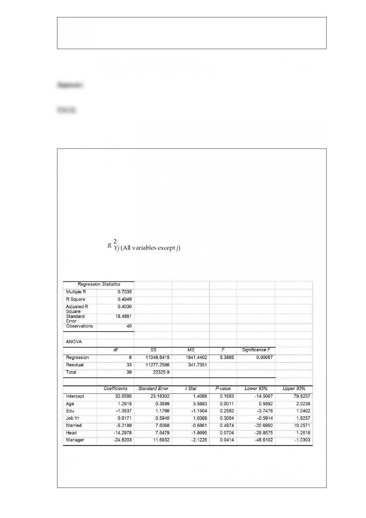
True or False: TABLE 17-10
Given below are results from the regression analysis where the dependent variable is
the number of weeks a worker is unemployed due to a layoff (Unemploy) and the
independent variables are the age of the worker (Age), the number of years of education
received (Edu), the number of years at the previous job (Job Yr), a dummy variable for
marital status (Married: 1 = married, 0 = otherwise), a dummy variable for head of
household (Head: 1 = yes, 0 = no) and a dummy variable for management position
(Manager: 1 = yes, 0 = no). We shall call this Model 1. The coefficient of partial
determination ( ) of each of the 6 predictors are, respectively,
0.2807, 0.0386, 0.0317, 0.0141, 0.0958, and 0.1201.
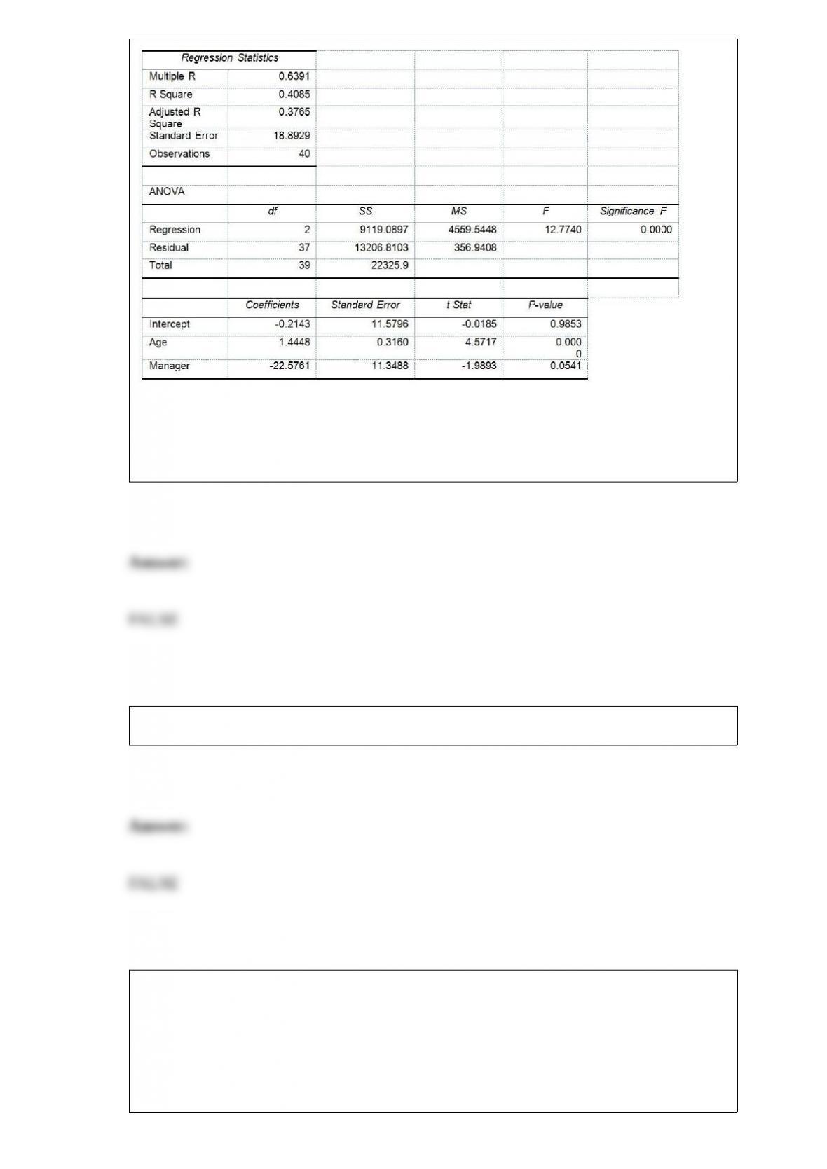
Model 2 is the regression analysis where the dependent variable is Unemploy and the
independent variables are Age and Manager. The results of the regression analysis are
given below:
Referring to Table 17-10, Model 1, the alternative hypothesis H1 : At least one of βj â
‰ 0 for j = 1, 2, 3, 4, 5, 6 implies that the number of weeks a worker is unemployed
due to a layoff is affected by all of the explanatory variables.
True or False: The median of the values 3.4, 4.7, 1.9, 7.6, and 6.5 is 1.9.
TABLE 8-5
A sample of salary offers (in thousands of dollars) given to management majors is: 48,
51, 46, 52, 47, 48, 47, 50, 51, and 59. Using this data to obtain a 95% confidence
interval resulted in an interval from 47.19 to 52.61.

True or False: Referring to Table 8-5, it is possible that the mean of the population is
between 47.19 and 52.61.
True or False: TABLE 17-10
Given below are results from the regression analysis where the dependent variable is
the number of weeks a worker is unemployed due to a layoff (Unemploy) and the
independent variables are the age of the worker (Age), the number of years of education
received (Edu), the number of years at the previous job (Job Yr), a dummy variable for
marital status (Married: 1 = married, 0 = otherwise), a dummy variable for head of
household (Head: 1 = yes, 0 = no) and a dummy variable for management position
(Manager: 1 = yes, 0 = no). We shall call this Model 1. The coefficient of partial
determination ( ) of each of the 6 predictors are, respectively,
0.2807, 0.0386, 0.0317, 0.0141, 0.0958, and 0.1201.
Model 2 is the regression analysis where the dependent variable is Unemploy and the
independent variables are Age and Manager. The results of the regression analysis are
given below:
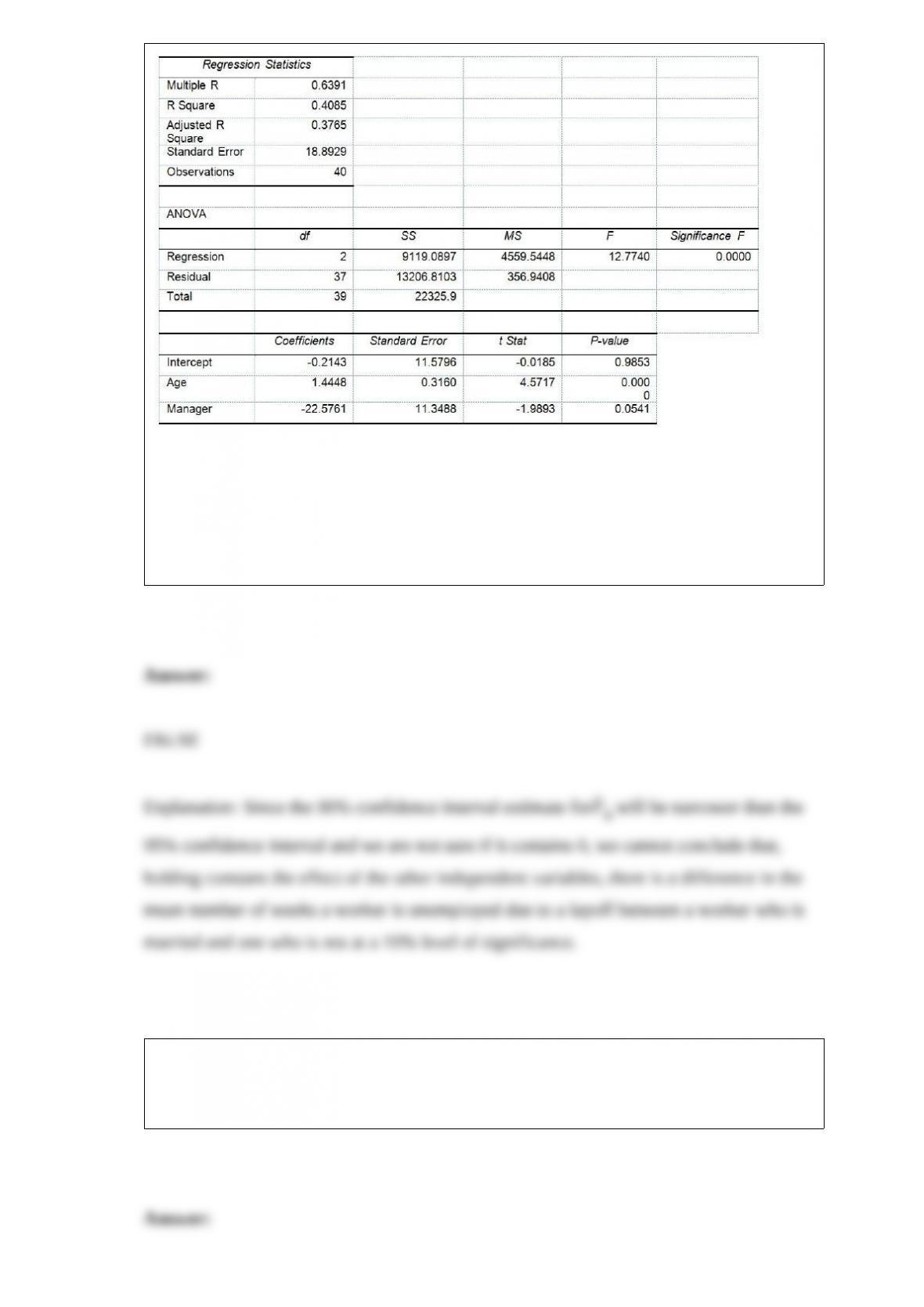
Referring to Table 17-10, Model 1, we can conclude that, holding constant the effect of
the other independent variables, there is a difference in the mean number of weeks a
worker is unemployed due to a layoff between a worker who is married and one who is
not at a 10% level of significance if we use only the information of the 95% confidence
interval estimate forβ4.
True or False: An electronic appliance chain gathered customer opinions on their
services using the customer feedback forms that are attached to the product registration
forms. This is an example of a convenience sample.
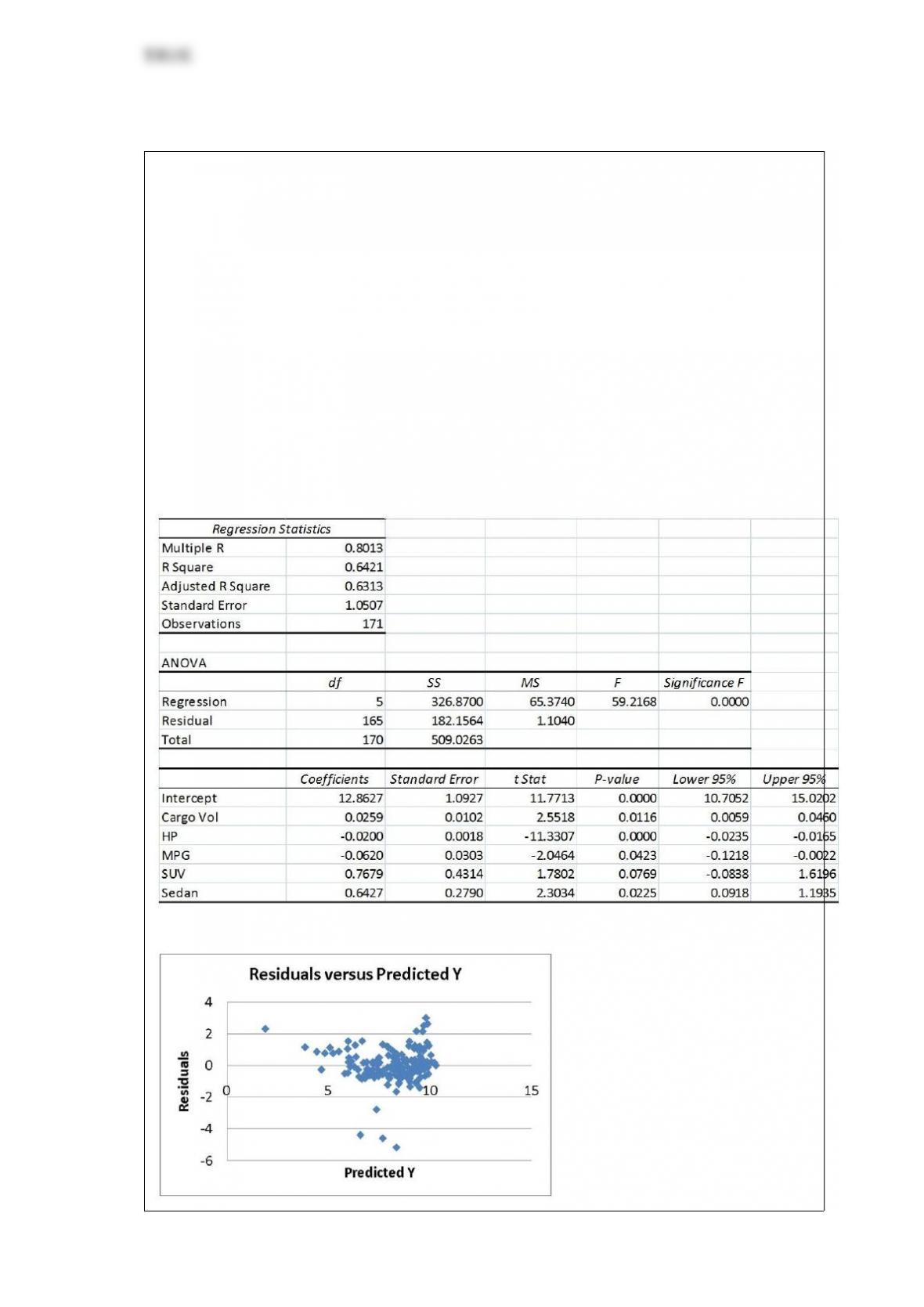
True or False: TABLE 17-9
What are the factors that determine the acceleration time (in sec.) from 0 to 60 miles per
hour of a car? Data on the following variables for 171 different vehicle models were
collected:
Accel Time: Acceleration time in sec.
Cargo Vol: Cargo volume in cu. ft.
HP: Horsepower
MPG: Miles per gallon
SUV: 1 if the vehicle model is an SUV with Coupe as the base when SUV and Sedan
are both 0
Sedan: 1 if the vehicle model is a sedan with Coupe as the base when SUV and Sedan
are both 0
The regression results using acceleration time as the dependent variable and the
remaining variables as the independent variables are presented below.
The various residual plots are as shown below.
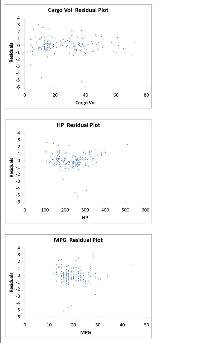
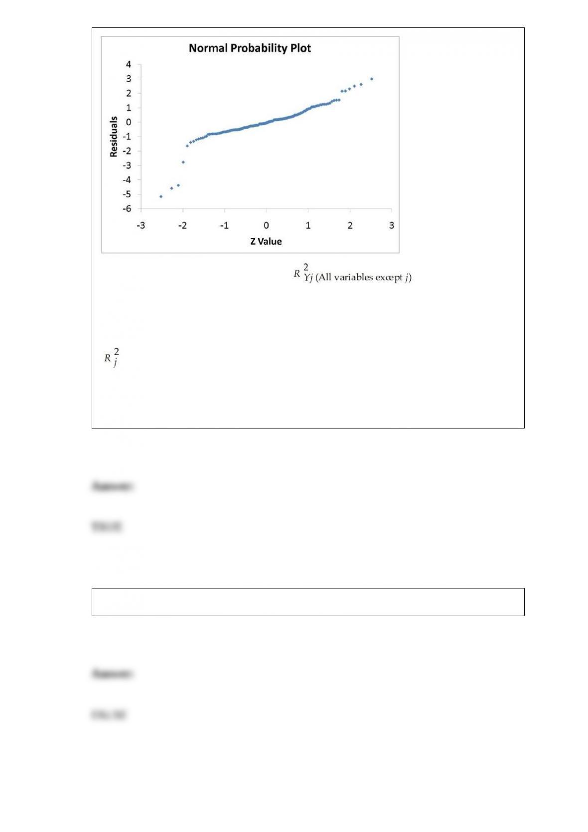
The coefficient of partial determination ( ) of each of the 5
predictors are, respectively, 0.0380, 0.4376, 0.0248, 0.0188, and 0.0312.
The coefficient of multiple determination for the regression model using each of the 5
variables Xj as the dependent variable and all other X variables as independent variables
( ) are, respectively, 0.7461, 0.5676, 0.6764, 0.8582, 0.6632.
Referring to Table 17-9, there is enough evidence to conclude that Cargo Vol makes a
significant contribution to the regression model in the presence of the other independent
variables at a 5% level of significance.
True or False: If P(A) = 0.4 and P(B) = 0.6, then A and B must be mutually exclusive.
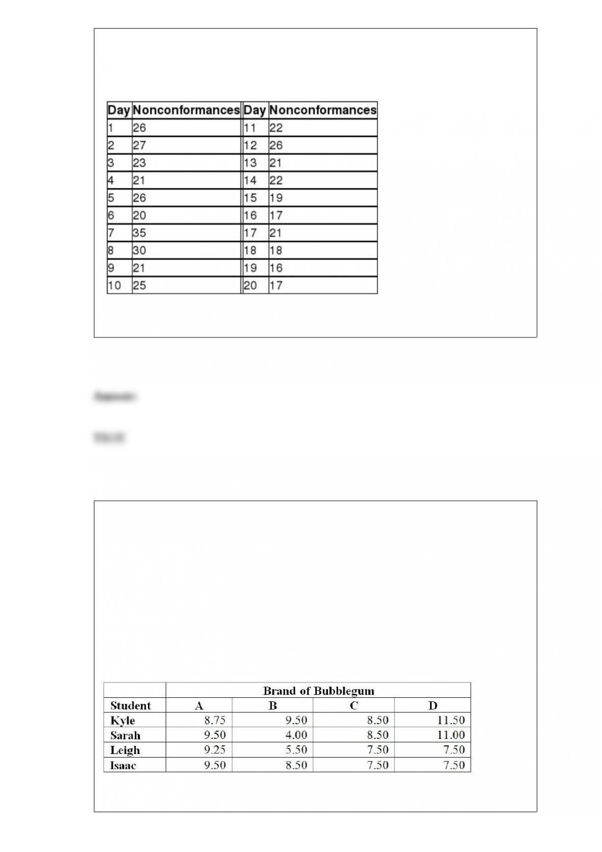
True or False: TABLE 18-10
Below is the number of defective items from a production line over twenty consecutive
morning shifts.
Referring to Table 18-10, based on the c chart, there appears to be a special cause of
variation in the process.
TABLE 11-11
A student team in a business statistics course designed an experiment to investigate
whether the brand of bubblegum used affected the size of bubbles they could blow. To
reduce the person-to-person variability, the students decided to use a randomized block
design using themselves as blocks.
Four brands of bubblegum were tested. A student chewed two pieces of a brand of gum
and then blew a bubble, attempting to make it as big as possible. Another student
measured the diameter of the bubble at its biggest point. The following table gives the
diameters of the bubbles (in inches) for the 16 observations.
True or False: Referring to Table 11-11, the relative efficiency means that 1.0144 times

as many observations in each brand would be needed in a one-way ANOVA design as
compared to the randomized block design in order to obtain the same precision for
comparison of the different means.
The residuals represent
A) the difference between the actual Y values and the mean of Y.
B) the difference between the actual Y values and the predicted Y values.
C) the square root of the slope.
D) the predicted value of Y for the average X value.
Data on the amount of money made in a year by 1,000 families in a small town were
collected. You want to know the difference in the amount of money made in that year
by the middle 50% of the 1,000 families. Which of the following would you compute?
A) Arithmetic mean
B) Median
C) Interquartile range
D) Coefficient of correlation
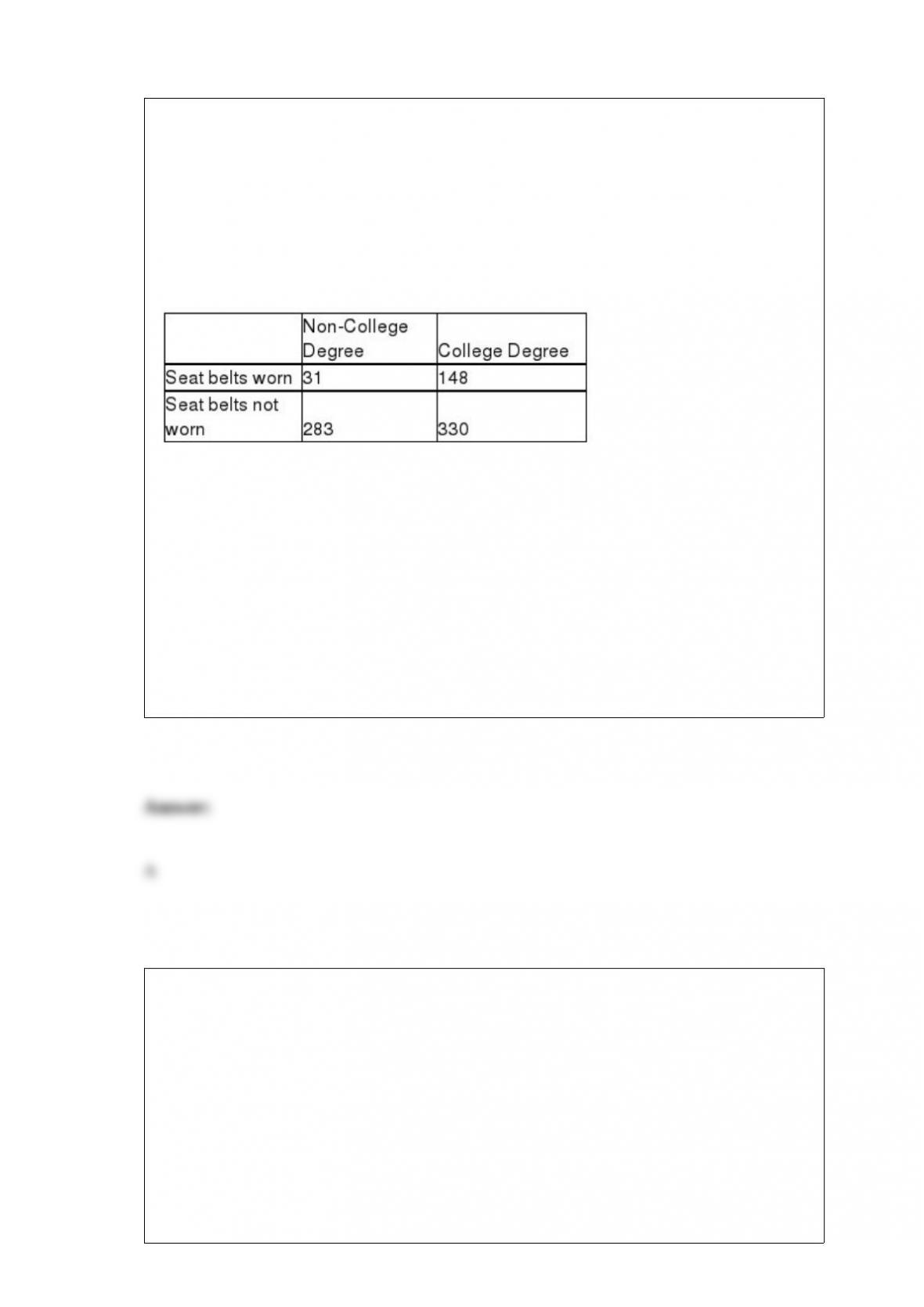
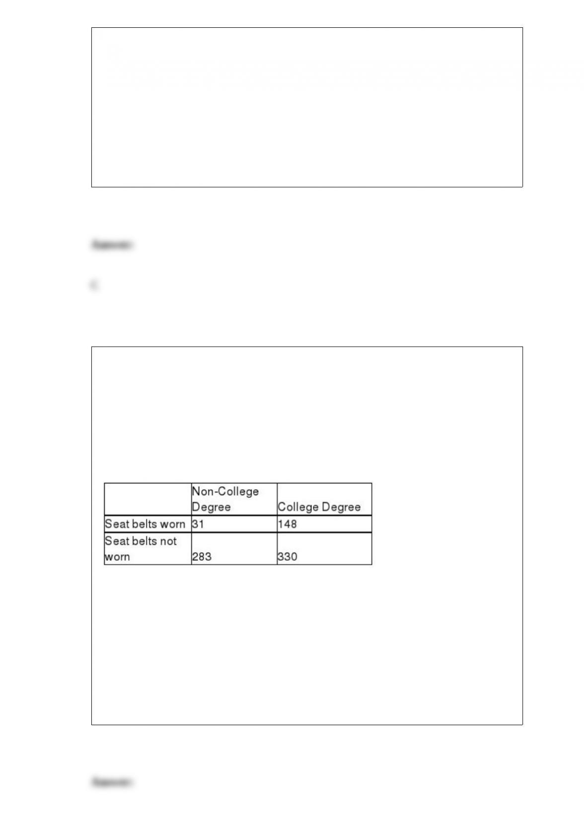
TABLE 12-8
A study was conducted to determine whether the use of seat belts in motor vehicles
depends on the educational status of the parents. A sample of 792 children treated for
injuries sustained from motor vehicle accidents was obtained, and each child was
classified according to (1) parents’ educational status (College Degree or Non-College
Degree) and (2) seat belt usage (worn or not worn) during the accident. The number of
children in each category is given in the table below.
Referring to Table 12-8, at 5% level of significance, the critical value of the test statistic
is
A) 3.8415.
B) 5.9914.
C) 9.4877.
D) 13.2767.
Every spring semester, the School of Business coordinates with local business leaders a
luncheon for graduating seniors, their families, and friends. Corporate sponsorship pays
for the lunches of each of the seniors, but students have to purchase tickets to cover the
cost of lunches served to guests they bring with them. Data on the number of guests
each graduating senior invited to the luncheon from 500 graduating seniors last year
were collected. Based on this information, which of the following will you construct to
learn about the percentage of seniors who will bring at least one guest to the luncheon?
A) Confidence interval estimate for the total using the Student’s t distribution
B) Confidence interval estimate for the mean using the Student’s t distribution
C) Confidence interval estimate for the proportion using the standard normal
distribution
D) Confidence interval estimate for the difference between two means using the
standard normal distribution
For a potential investment of $5,000, a portfolio has an EMV of $1,000 and a standard
deviation of $100. The return to risk ratio is
A) 50.
B) 20.
C) 10.
D) 5.
In testing for differences between the means of two independent populations, the null
hypothesis is
A) H0 : 1 – 2 = 2.
B) H0 : 1 – 2 = 0.
C) H0 : 1 – 2 > 0.
D) H0 : 1 – 2 < 2.
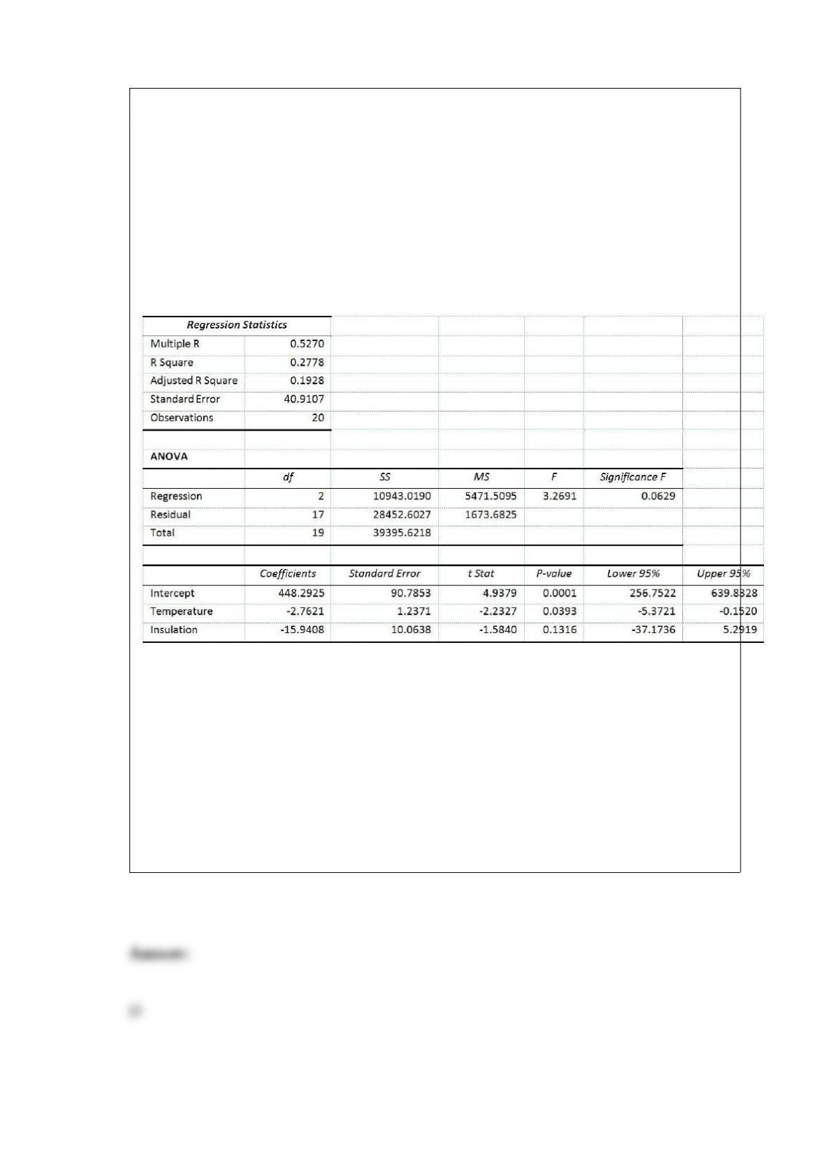
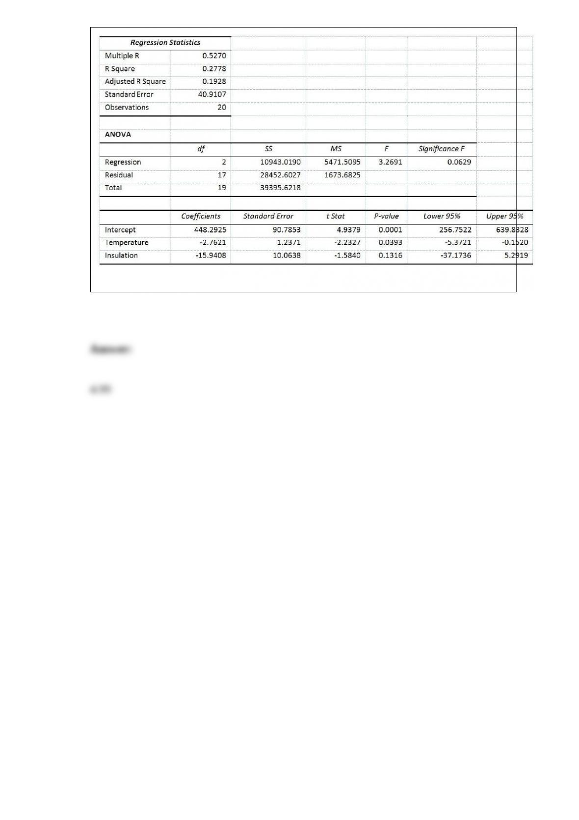
Referring to Table 14-6, what is your decision and conclusion for the test H0 : β2 = 0
vs. H1 : β2 ≠0 at the α = 0.01 level of significance?
TABLE 14-6
One of the most common questions of prospective house buyers pertains to the cost of
heating in dollars (Y). To provide its customers with information on that matter, a large
real estate firm used the following 2 variables to predict heating costs: the daily
minimum outside temperature in degrees of Fahrenheit (X1) and the amount of
insulation in inches (X2). Given below is EXCEL output of the regression model.
Also SSR (X1∣ X2) = 8343.3572 and SSR (X2∣ X1) = 4199.2672
A) Do not reject H0 and conclude that the amount of insulation has a linear effect on
heating costs.
B) Reject H0 and conclude that the amount of insulation does not have a linear effect on
heating costs.
C) Reject H0 and conclude that the amount of insulation has a linear effect on heating
costs.
D) Do not reject H0 and conclude that the amount of insulation does not have a linear
effect on heating costs.
Which of the following assumptions concerning the probability distribution of the
random error term is stated incorrectly?
A) The distribution is normal.
B) The mean of the distribution is 0.
C) The variance of the distribution increases as X increases.
D) The errors are independent.
TABLE 12-8
A study was conducted to determine whether the use of seat belts in motor vehicles
depends on the educational status of the parents. A sample of 792 children treated for
injuries sustained from motor vehicle accidents was obtained, and each child was
classified according to (1) parents’ educational status (College Degree or Non-College
Degree) and (2) seat belt usage (worn or not worn) during the accident. The number of
children in each category is given in the table below.
Referring to Table 12-8, the calculated test statistic is
A) -0.9991.
B) -0.1368.
C) 48.1849.
D) 72.8063.
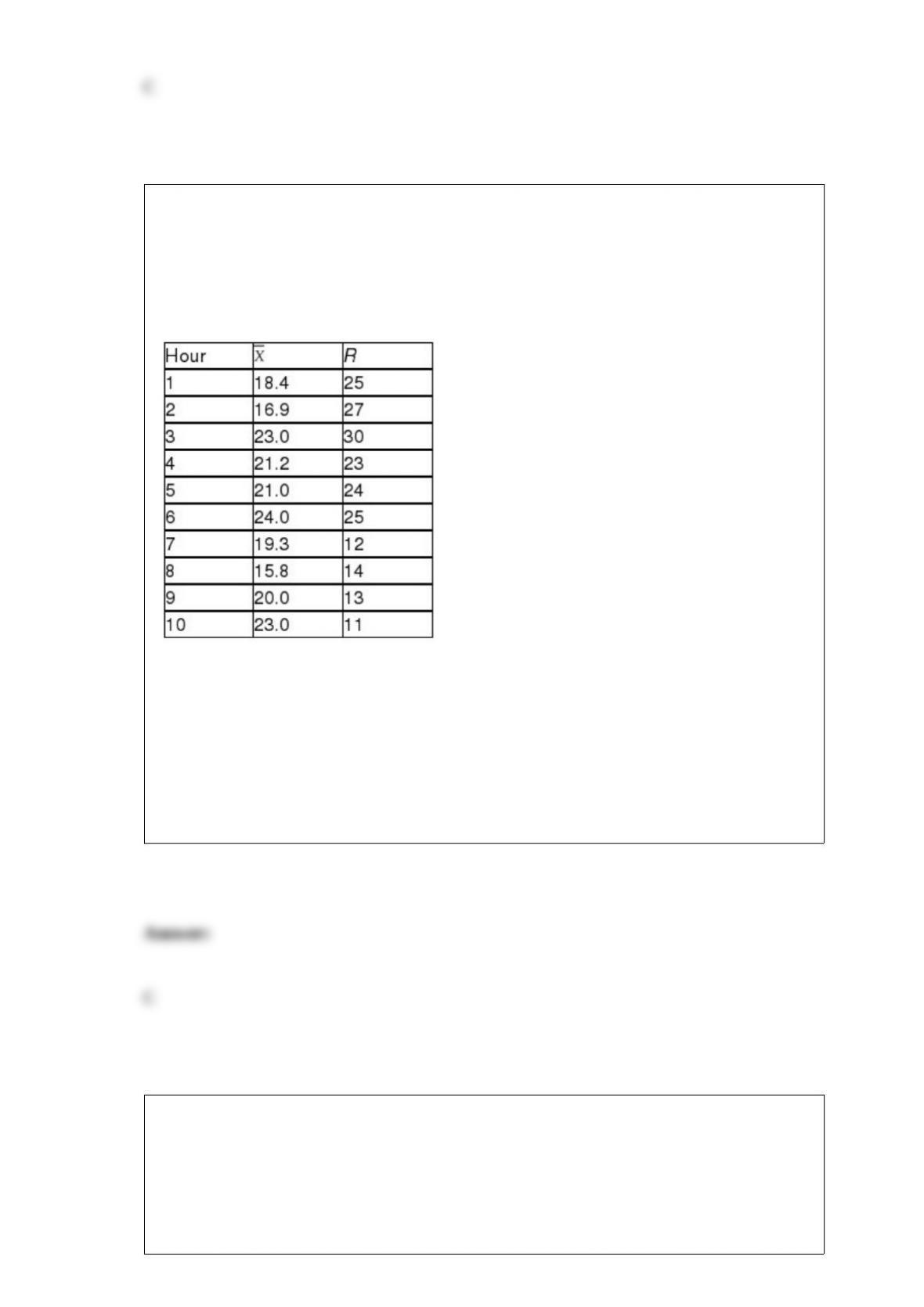
TABLE 18-4
A factory supervisor is concerned that the time it takes workers to complete an
important production task (measured in seconds) is too erratic and adversely affects
expected profits. The supervisor proceeds by randomly sampling 5 individuals per hour
for a period of 10 hours. The sample mean and range for each hour are listed below.
She also decides that lower and upper specification limit for the critical-to-quality
variable should be 10 and 30 seconds, respectively.
Referring to Table 18-4, suppose the supervisor constructs an R chart to see if the
variability in collection times is in-control. What is the center line of this R chart?
A) 20.00
B) 20.56
C) 20.40
D) 24.00
TABLE 2-2
At a meeting of information systems officers for regional offices of a national company,
a survey was taken to determine the number of employees the officers supervise in the
operation of their departments, where X is the number of employees overseen by each
information systems officer.
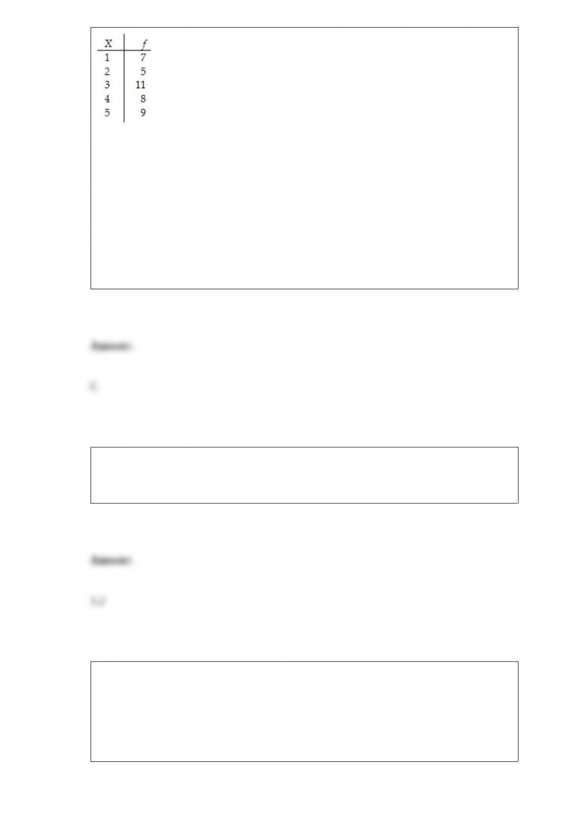
Referring to Table 2-2, across all of the regional offices, how many total employees
were supervised by those surveyed?
A) 15
B) 40
C) 127
D) 200
Suppose that past history shows that 60% of college students prefer Brand C cola. A
sample of 5 students is to be selected. The variance of the number that prefer brand C is
________.
TABLE 12-18
The director of transportation of a large company is interested in the usage of the
company’s van pool program. She surveyed 129 of her employees on the usage of the
program before and after a campaign to convince her employees to use the service and
obtained the following:

She will use this information to perform a test using a level of significance of 0.05.
Referring to Table 12-18, the director now wants to know if the proportion of
employees who use the service before the campaign and the proportion of employees
who use the service after the campaign are the same. What should be her conclusion?
A) There is sufficient evidence that the proportion of employees who use the service
before the campaign is the same as the proportion of employees who use the service
after the campaign.
B) There is insufficient evidence that the proportion of employees who use the service
before the campaign is the same as the proportion of employees who use the service
after the campaign.
C) There is sufficient evidence that the proportion of employees who use the service
before the campaign is not the same as the proportion of employees who use the service
after the campaign.
D) There is insufficient evidence that the proportion of employees who use the service
before the campaign is not the same as the proportion of employees who use the service
after the campaign.
In a multiple regression model, which of the following is correct regarding the value of
the adjusted r2?
A) It can be negative.
B) It has to be positive.
C) It has to be larger than the coefficient of multiple determination.
D) It can be larger than 1.
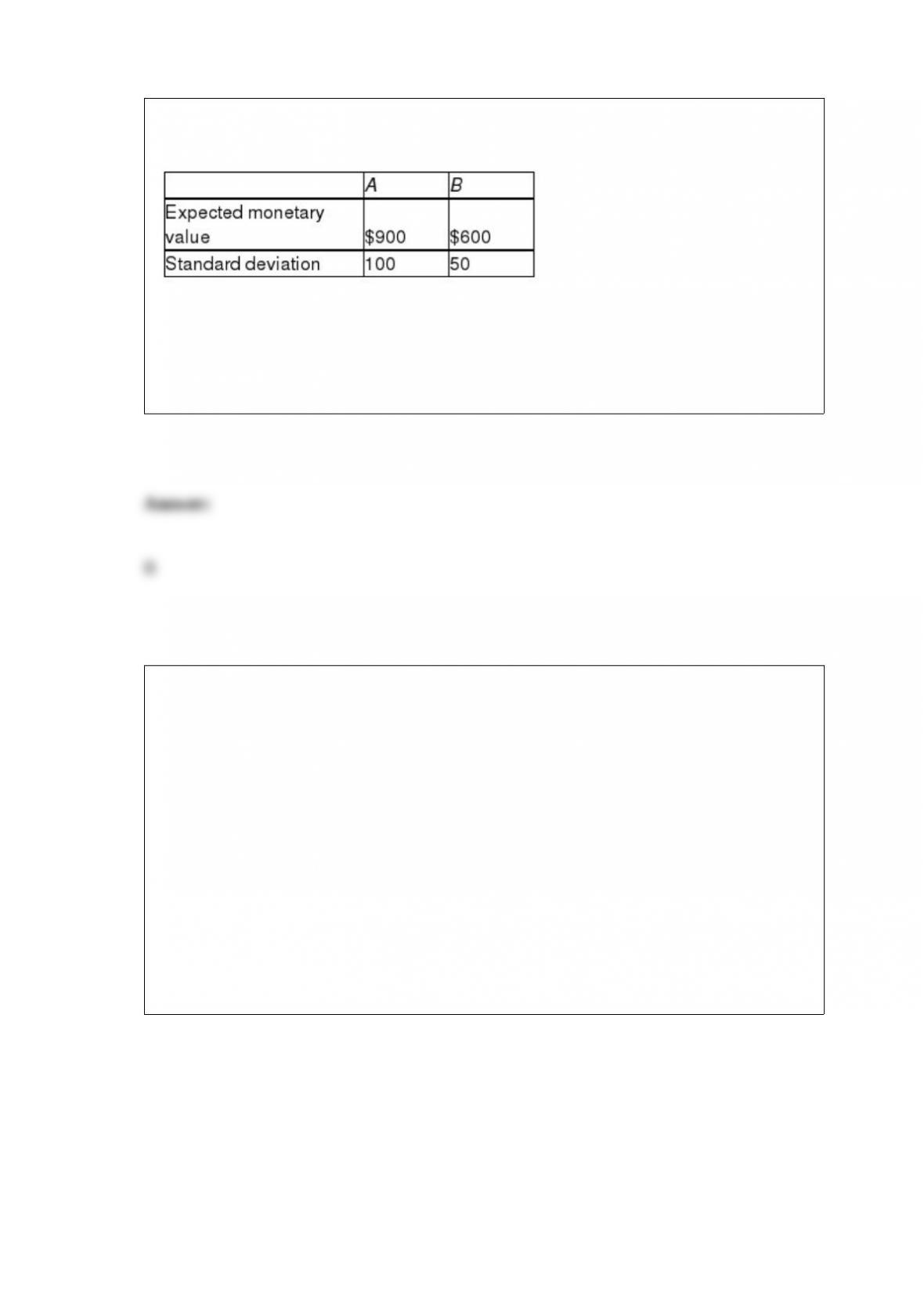
TABLE 19-3
The following information is from 2 investment opportunities.
Referring to Table 19-3, which investment has the optimal coefficient of variation?
A) Investment A
B) Investment B
C) The investments are equal.
D) It cannot be determined.
Referring to Table 14-17, which of the following is the correct
alternative hypothesis to test whether age has any effect on the
number of weeks a worker is unemployed due to a layoff while
holding constant the effect of the other independent variable?
TABLE 14-17
Given below are results from the regression analysis where the
dependent variable is the number of weeks a worker is unemployed
due to a layoff (Unemploy) and the independent variables are the age
of the worker (Age) and a dummy variable for management position
(Manager: 1 = yes, 0 = no).
The results of the regression analysis are given below:

A) H1 : β1 = 0
B) H1 : β1 ≠0
C) H1 : β2 = 0
D) H1 : β2 ≠0
TABLE 16-13
Given below is the monthly time-series data for U.S. retail sales of building materials
over a specific year.
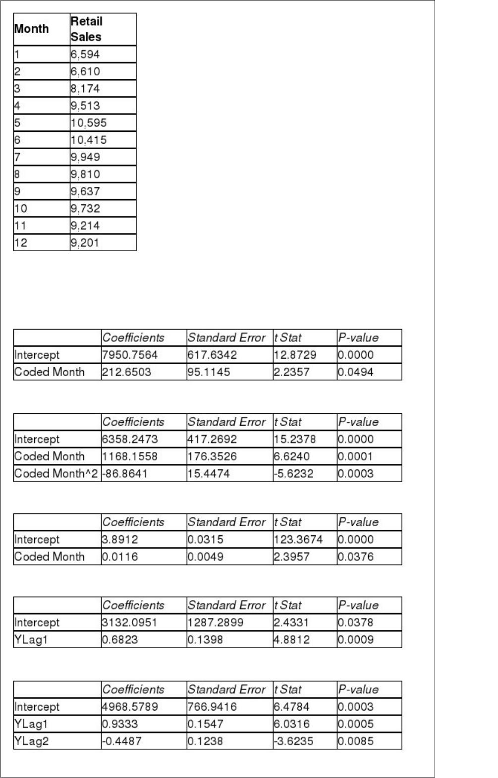
The results of the linear trend, quadratic trend, exponential trend, first-order
autoregressive, second-order autoregressive and third-order autoregressive model are
presented below in which the coded month for the 1st month is 0:
Linear trend model:
Quadratic trend model:
Exponential trend model:
First-order autoregressive:
Second-order autoregressive:
Third-order autoregressive:
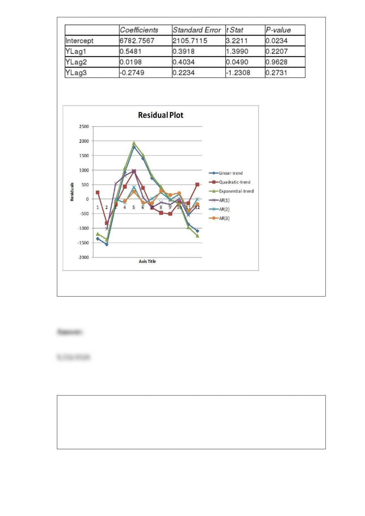
Below is the residual plot of the various models:
Referring to Table 16-13, what is your forecast for the 13th month using the third-order
autoregressive model?
TABLE 3-8
The time period from 2009 to 2012 saw a great deal of volatility in the value of stocks.
The data in the following table represent the total rate of return of our companies from
2009 to 2012.
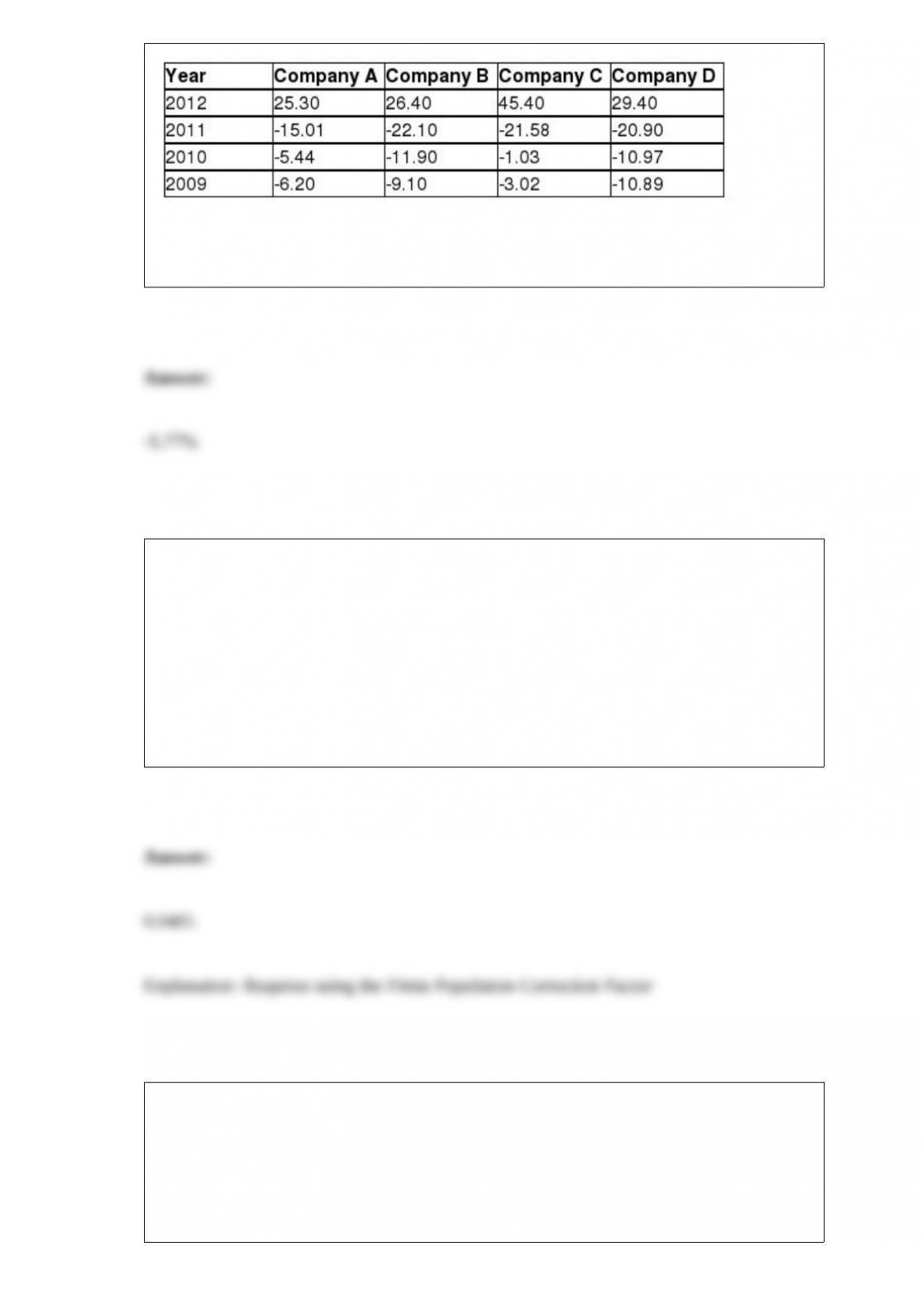
Referring to Table 3-8, calculate the geometric mean rate of return per year for
Company B.
TABLE 8-15
The president of a university is concerned that illicit drug use on campus is higher than
the 5% targeted level. A random sample of 250 students from a population of 2,000
revealed that 7 of them had used illicit drugs during the last 12 months.
Referring to Table 8-15, what is the upper bound of the 90% one-sided confidence
interval for the proportion of students who had used illicit drugs during the last 12
months?
TABLE 5-2
A certain type of new business succeeds 60% of the time. Suppose that 3 such
businesses open (where they do not compete with each other, so it is reasonable to
believe that their relative successes would be independent).
Referring to Table 5-2, the probability that all 3 businesses succeed is ________.
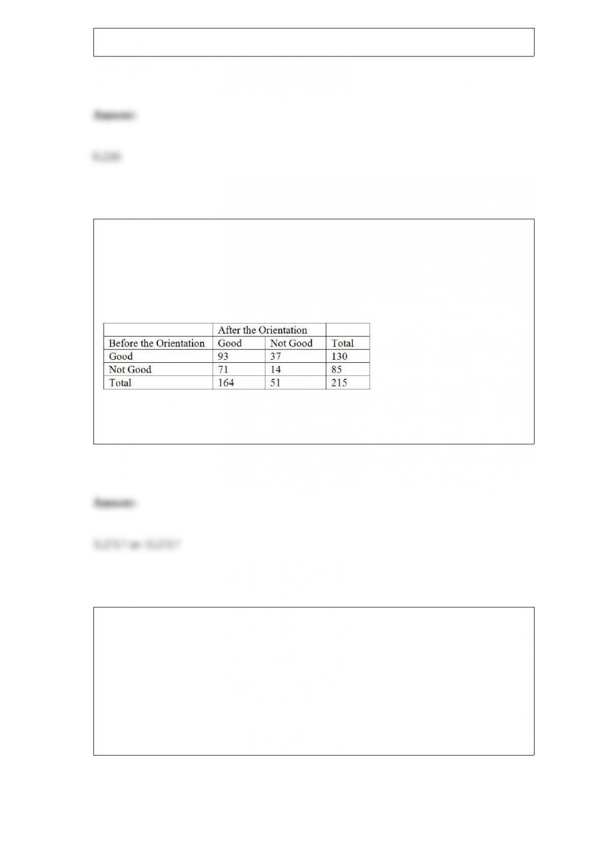
TABLE 12-19
The director of the MBA program of a state university wanted to know if a one-week
orientation would change the proportion among potential incoming students who would
perceive the program as being good. Given below is the result from 215 students’ view
of the program before and after the orientation.
Referring to Table 12-19, what is the value of the test statistic using a 1% level of
significance?
TABLE 4-5
In a meat packaging plant Machine A accounts for 60% of the plant’s output, while
Machine B accounts for 40% of the plant’s output. In total, 4% of the packages are
improperly sealed. Also, 3% of the packages are from Machine A and are improperly
sealed.
Referring to Table 4-5, if a package selected at random came from Machine B, the
probability that it is properly sealed is ________.
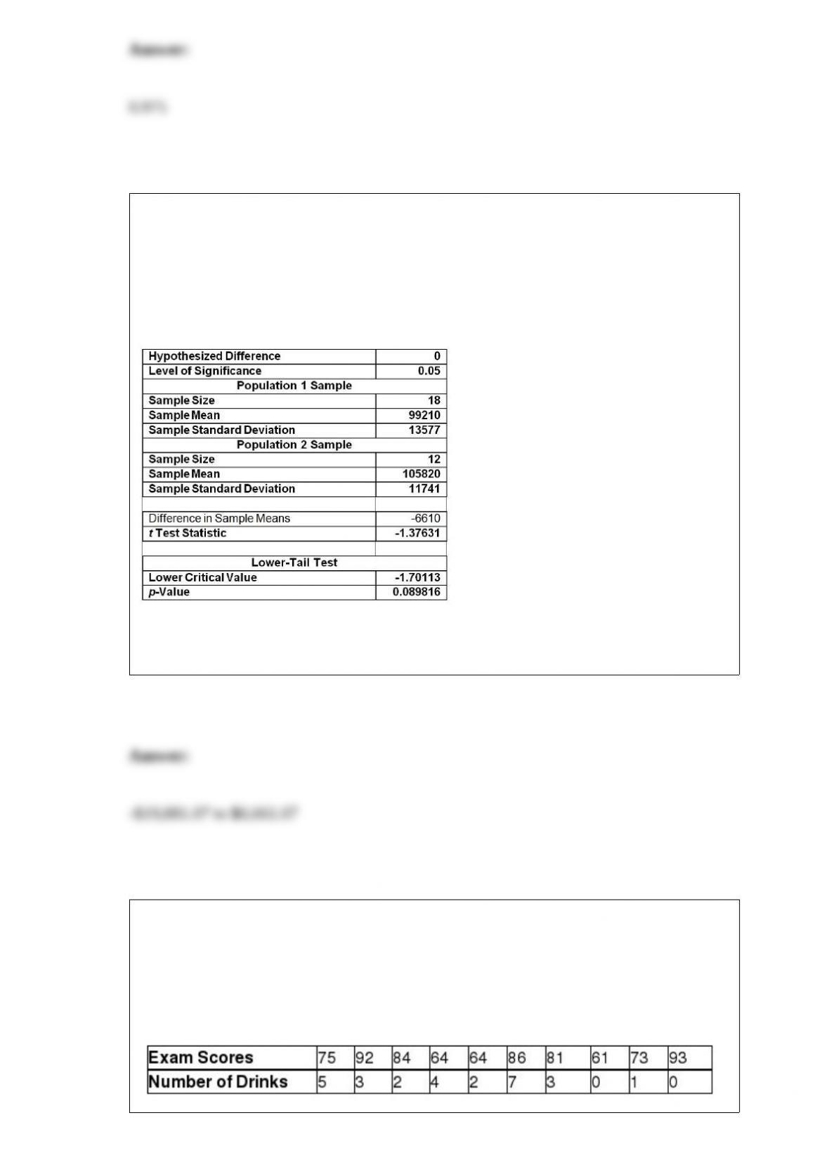
TABLE 10-2
A researcher randomly sampled 30 graduates of an MBA program and recorded data
concerning their starting salaries. Of primary interest to the researcher was the effect of
gender on starting salaries. The result of the pooled-variance t-test of the mean salaries
of the females (Population 1) and males (Population 2) in the sample is given below.
Referring to Table 10-2, what is the 99% confidence interval estimate for the difference
between two means?
TABLE 3-13
Energy drink consumption has continued to gain in popularity since the 1997 debut of
Red Bull, the current leader in the energy drink market. Given below are the exam
scores and the number of 12-ounce energy drinks consumed within a week prior to the
exam of 10 college students.
Referring to Table 3-13, what is the sample correlation coefficient between the exam
scores and the number of energy drinks consumed?
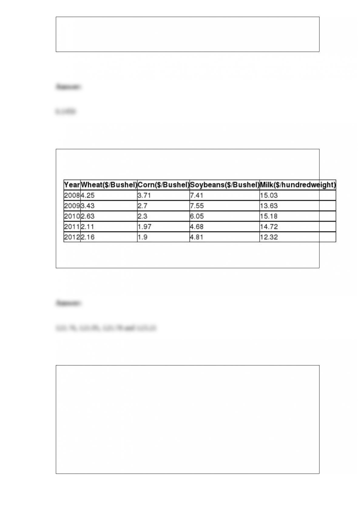
TABLE 16-16
Given below are the prices of a basket of four food items from 2008 to 2012.
Referring to Table 16-16, what are the simple price indices for wheat, corn, soybeans
and milk, respectively, in 2010 using 2012 as the base year?
Referring to Table 14-6, the value of the partial F test statistic is ________ for
H0: Variable X1 does not significantly improve the model after variable X2 has been
included
H1 : Variable X1 significantly improves the model after variable X2 has been included
TABLE 14-6
One of the most common questions of prospective house buyers pertains to the cost of
heating in dollars (Y). To provide its customers with information on that matter, a large
real estate firm used the following 2 variables to predict heating costs: the daily
minimum outside temperature in degrees of Fahrenheit (X1) and the amount of
insulation in inches (X2). Given below is EXCEL output of the regression model.
Also SSR (X1∣ X2) = 8343.3572 and SSR (X2∣ X1) = 4199.2672