TABLE 9-6
The quality control engineer for a furniture manufacturer is interested in the mean
amount of force necessary to produce cracks in stressed oak furniture. She performs a
two-tail test of the null hypothesis that the mean for the stressed oak furniture is 650.
The calculated value of the Z test statistic is a positive number that leads to a p-value of
0.080 for the test.
True or False: Referring to Table 9-6, suppose the engineer had decided that the
alternative hypothesis to test was that the mean was greater than 650. Then if the test is
performed with a level of significance of 0.05, the null hypothesis would be rejected.
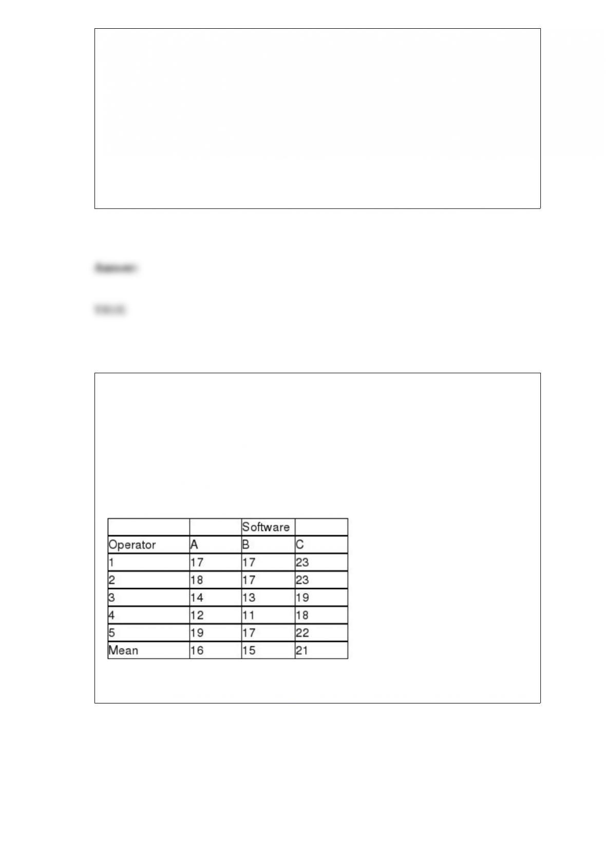
TABLE 11-8
An important factor in selecting database software is the time required for a user to
learn how to use the system. To evaluate three potential brands (A, B and C) of database
software, a company designed a test involving five different employees. To reduce
variability due to differences among employees, each of the five employees is trained
on each of the three different brands. The amount of time (in hours) needed to learn
each of the three different brands is given below:
Below is the Excel output for the randomized block design:
True or False: Referring to Table 11-8, it is appropriate to use the Tukey multiple
comparison procedure based on the test result above.
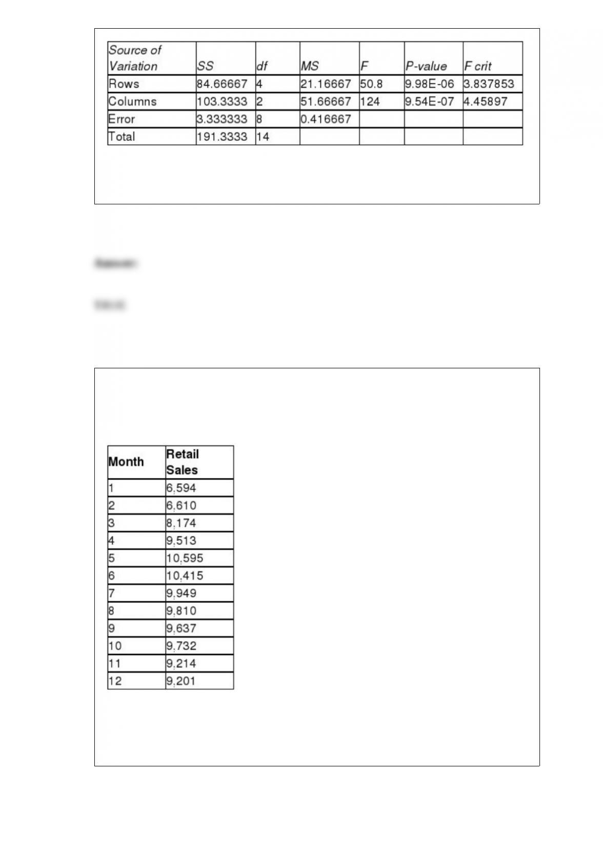
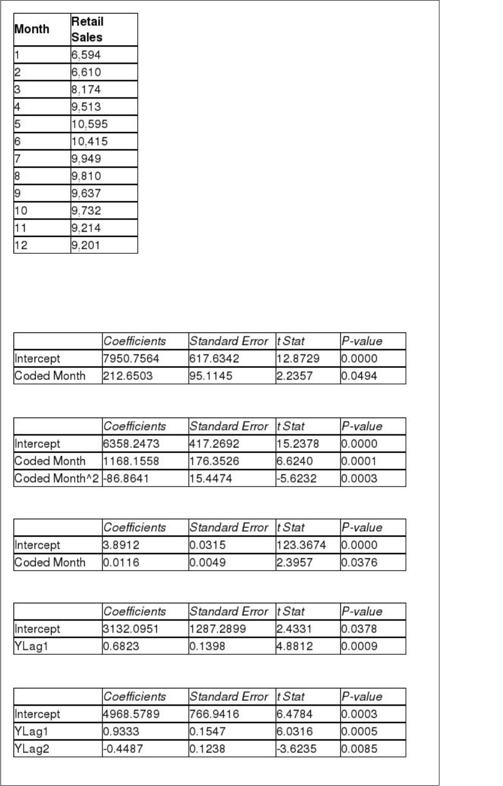
TABLE 16-13
Given below is the monthly time-series data for U.S. retail sales of building materials
over a specific year.
The results of the linear trend, quadratic trend, exponential trend, first-order
autoregressive, second-order autoregressive and third-order autoregressive model are
presented below in which the coded month for the 1st month is 0:
Linear trend model:
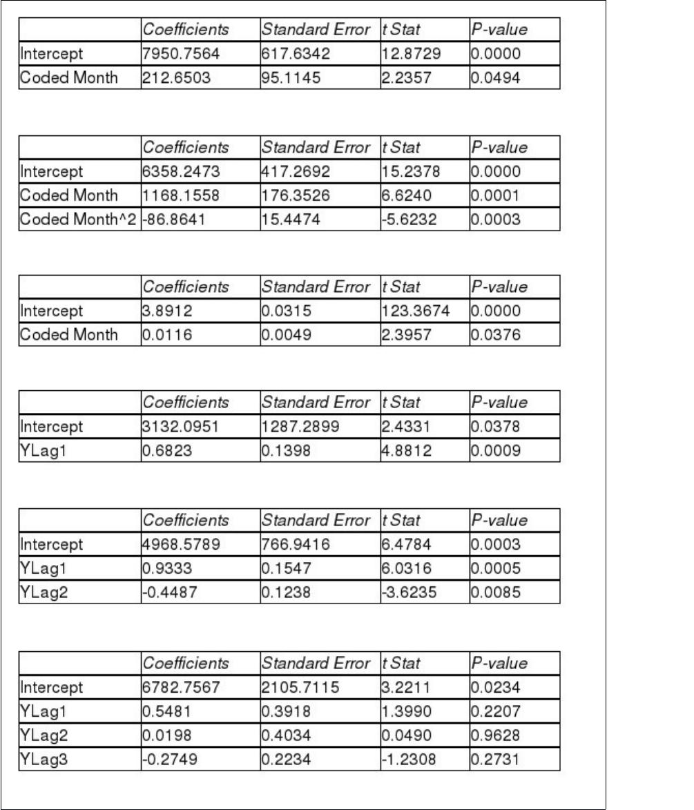
Quadratic trend model:
Exponential trend model:
First-order autoregressive:
Second-order autoregressive:
Third-order autoregressive:
Below is the residual plot of the various models:
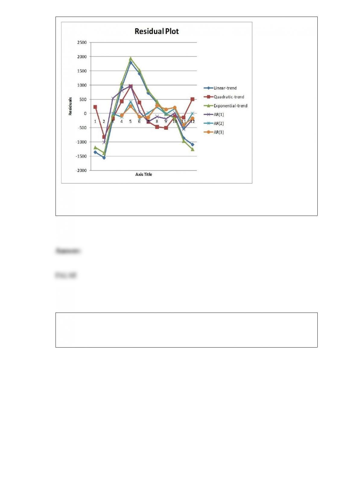
True or False: Referring to Table 16-13, you can reject the null hypothesis for testing
the appropriateness of the third-order autoregressive model at the 5% level of
significance.
TABLE 16-13
Given below is the monthly time-series data for U.S. retail sales of building materials
over a specific year.
The results of the linear trend, quadratic trend, exponential trend, first-order
autoregressive, second-order autoregressive and third-order autoregressive model are
presented below in which the coded month for the 1st month is 0:
Linear trend model:
Quadratic trend model:
Exponential trend model:
First-order autoregressive:
Second-order autoregressive:
Third-order autoregressive:
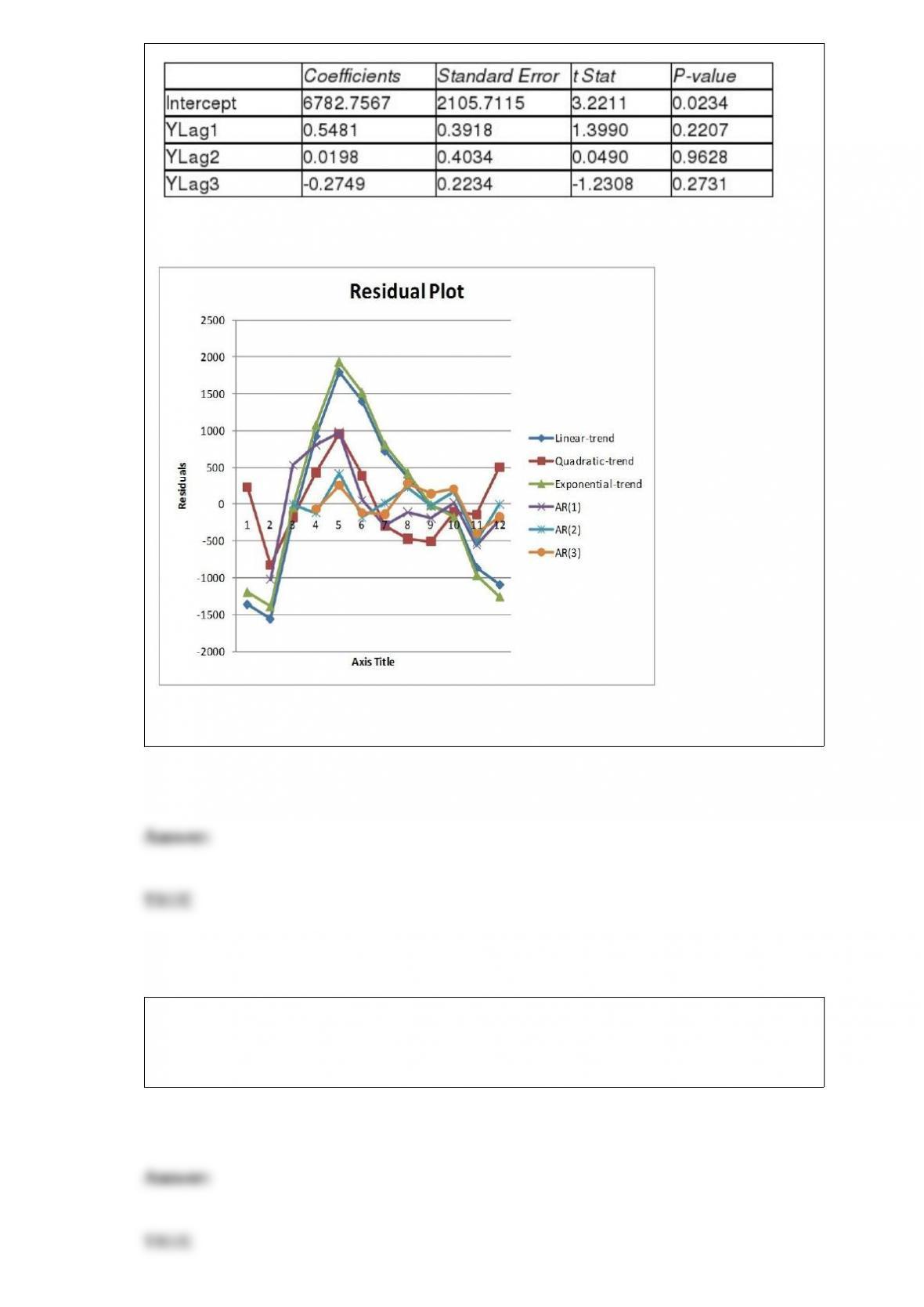
Below is the residual plot of the various models:
True or False: Referring to Table 16-13, the best model based on the residual plots is the
second-order autoregressive model.
True or False: The variance of the sum of two investments will be equal to the sum of
the variances of the two investments when the covariance between the investments is
zero.
True or False: The R chart is a control chart used to monitor a process mean.
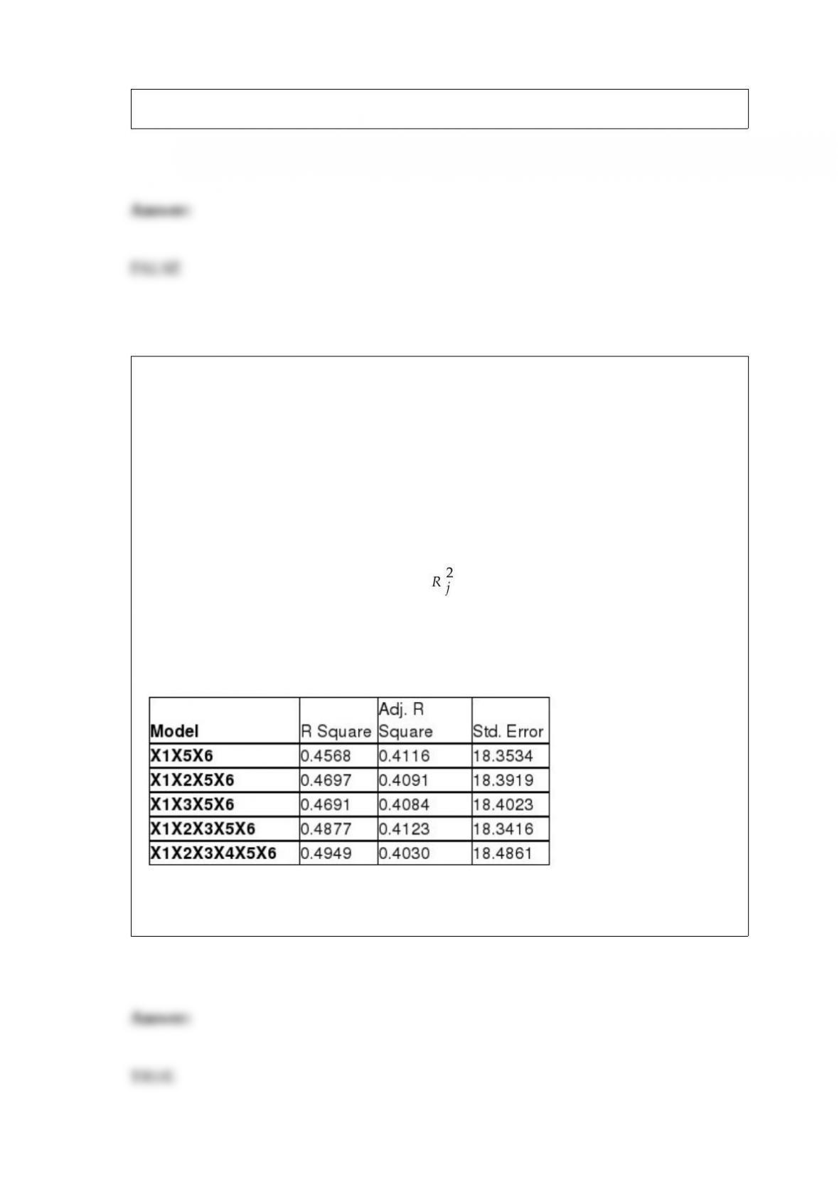
TABLE 15-6
Given below are results from the regression analysis on 40 observations where the
dependent variable is the number of weeks a worker is unemployed due to a layoff (Y)
and the independent variables are the age of the worker (X1), the number of years of
education received (X2), the number of years at the previous job (X3), a dummy variable
for marital status (X4: 1 = married, 0 = otherwise), a dummy variable for head of
household (X5: 1 = yes, 0 = no) and a dummy variable for management position (X6: 1
= yes, 0 = no).
The coefficient of multiple determination ( ) for the regression model using each of
the 6 variables Xj as the dependent variable and all other X variables as independent
variables are, respectively, 0.2628, 0.1240, 0.2404, 0.3510, 0.3342 and 0.0993.
The partial results from best-subset regression are given below:
True or False: Referring to Table 15-6, the model that includes X1, X2, X3, X5 and X6
should be selected using the adjusted r2 statistic.

True or False: TABLE 17-10
Given below are results from the regression analysis where the dependent variable is
the number of weeks a worker is unemployed due to a layoff (Unemploy) and the
independent variables are the age of the worker (Age), the number of years of education
received (Edu), the number of years at the previous job (Job Yr), a dummy variable for
marital status (Married: 1 = married, 0 = otherwise), a dummy variable for head of
household (Head: 1 = yes, 0 = no) and a dummy variable for management position
(Manager: 1 = yes, 0 = no). We shall call this Model 1. The coefficient of partial
determination ( ) of each of the 6 predictors are, respectively,
0.2807, 0.0386, 0.0317, 0.0141, 0.0958, and 0.1201.
Model 2 is the regression analysis where the dependent variable is Unemploy and the
independent variables are Age and Manager. The results of the regression analysis are
given below:
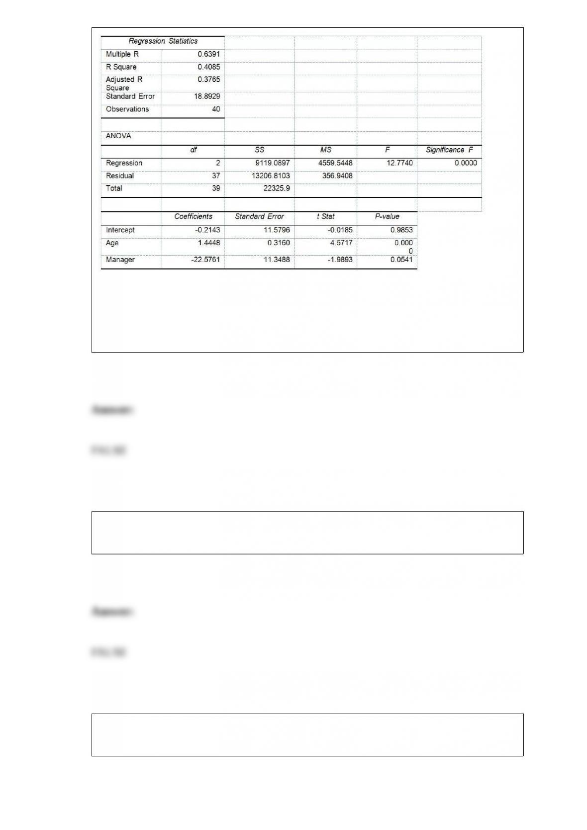
Referring to Table 17-10, Model 1, there is sufficient evidence that being married or not
makes a difference in the mean number of weeks a worker is unemployed due to a
layoff while holding constant the effect of all the other independent variables at a 10%
level of significance.
True or False: A histogram can have gaps between the bars, whereas bar charts cannot
have gaps.
True or False: A trend is a persistent pattern in annual time-series data that has to be
followed for several years.
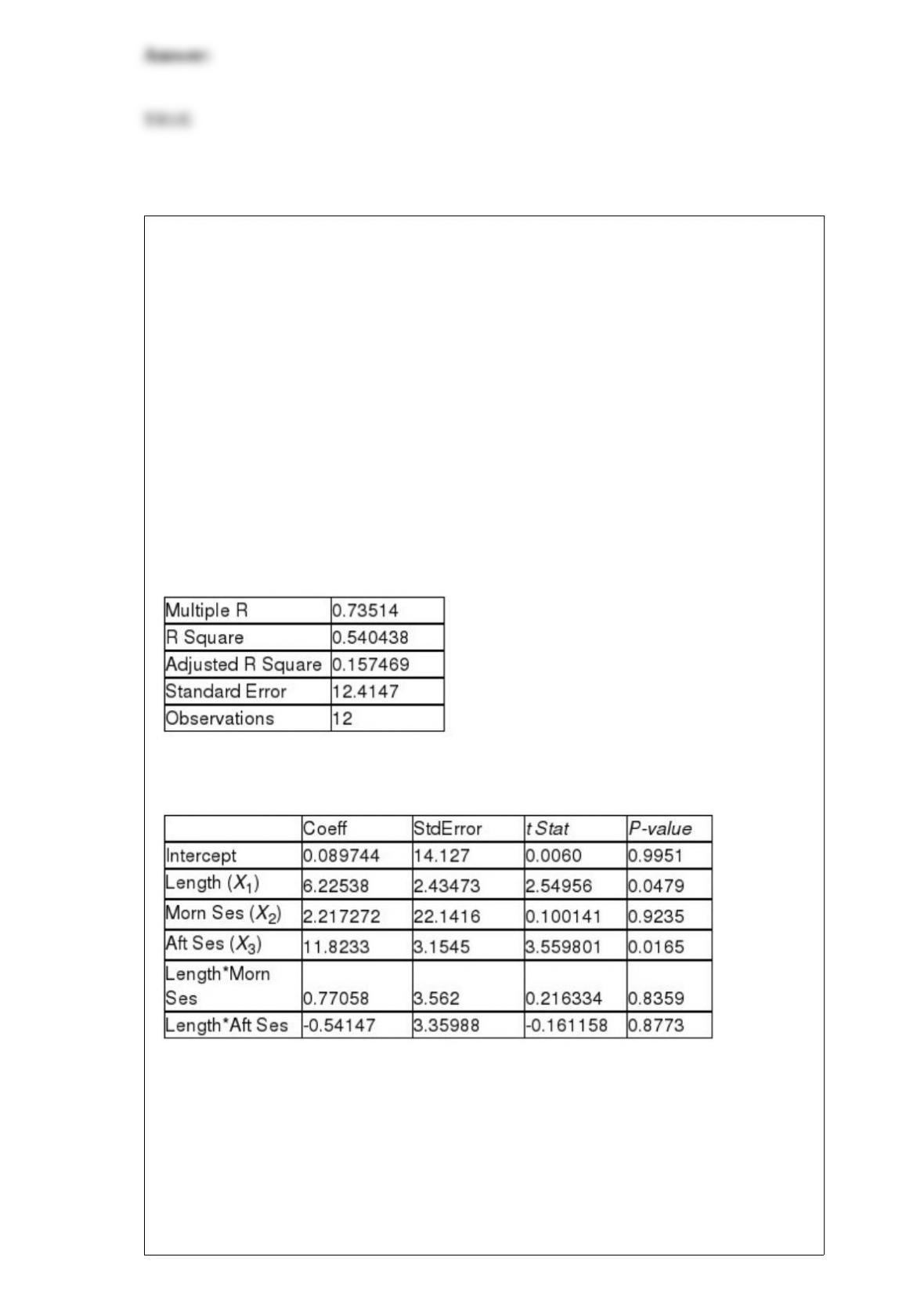
TABLE 17-6
A weight-loss clinic wants to use regression analysis to build a model for weight loss of
a client (measured in pounds). Two variables thought to affect weight loss are client’s
length of time on the weight-loss program and time of session. These variables are
described below:
Y = Weight loss (in pounds)
X1 = Length of time in weight-loss program (in months)
X2 = 1 if morning session, 0 if not
X3 = 1 if afternoon session, 0 if not (Base level = evening session)
Data for 12 clients on a weight-loss program at the clinic were collected and used to fit
the interaction model:
Y = β0 + β1X1 + β2X2 + β3X3 + β4X1X2 + β5X1X3 + ε
Partial output from Microsoft Excel follows:
Regression Statistics
ANOVA
F = 5.41118 Significance F = 0.040201
Referring to Table 17-6, in terms of the βs in the model, give the mean change in
weight loss (Y) for every 1-month increase in time in the program (X1) when attending
the afternoon session.
A) β1 + β4
B) β1 + β5
C) β1
D) β4 + β5
If the correlation coefficient (r) = 1.00, then
A) the Y-intercept (b0) must equal 0.
B) the explained variation equals the unexplained variation.
C) there is no unexplained variation.
D) there is no explained variation.
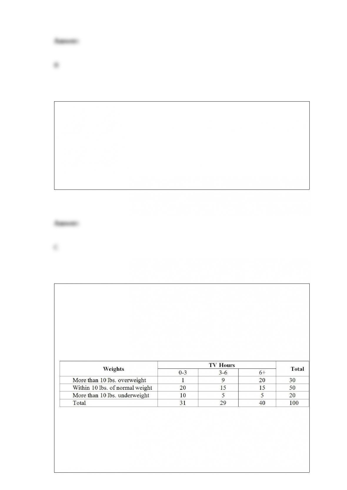
TABLE 12-13
Recent studies have found that American children are more obese than in the past. The
amount of time children spent watching television has received much of the blame. A
survey of 100 ten-year-olds revealed the following with regards to weights and average
number of hours a day spent watching television. We are interested in testing whether
the mean number of hours spent watching TV and weights are independent at 1% level
of significance.
Referring to Table 12-13, if there is no connection between weights and average
number of hours spent watching TV, we should expect how many children to be
spending no more than 6 hours on average watching TV and are more than 10 lbs.
underweight?
A) 5.8
B) 6.2
C) 8
D) 12
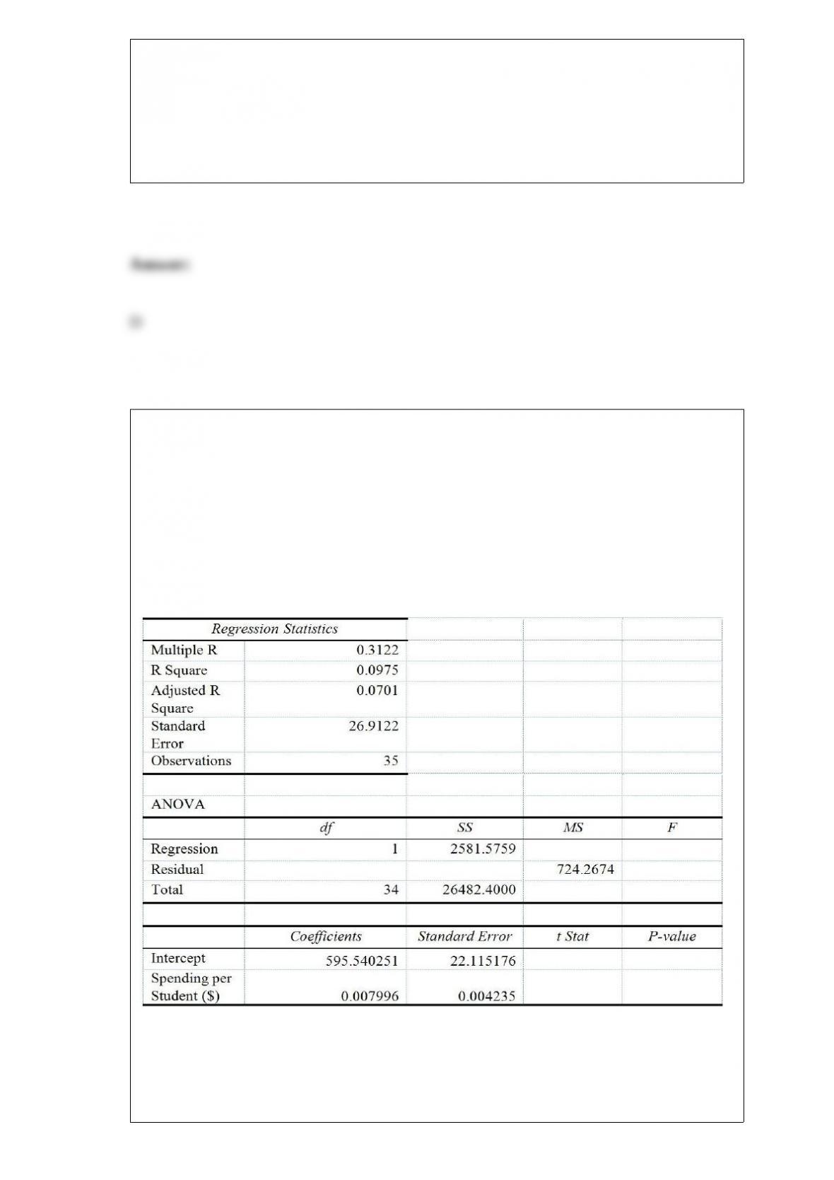
TABLE 13-13
In this era of tough economic conditions, voters increasingly ask the question: “Is the
educational achievement level of students dependent on the amount of money the state
in which they reside spends on education?” The partial computer output below is the
result of using spending per student ($) as the independent variable and composite score
which is the sum of the math, science and reading scores as the dependent variable on
35 states that participated in a study. The table includes only partial results.
Referring to Table 13-13, the conclusion on the test of whether spending per student
affects composite score using a 5% level of significance is that
A) there is not enough evidence that spending per student affects composite score.

B) there is enough evidence that spending per student affects composite score.
C) there is not enough evidence that spending per student does not affect composite
score.
D) there is enough evidence that spending per student does not affect composite score.
The owner of a local nightclub has recently surveyed a random sample of n = 250
customers of the club. She would now like to determine whether or not the mean age of
her customers is greater than 30. If so, she plans to alter the entertainment to appeal to
an older crowd. If not, no entertainment changes will be made. Suppose she found that
the sample mean was 30.45 years and the sample standard deviation was 5 years. If she
wants to have a level of significance at 0.01 what conclusion can she make?
A) There is not sufficient evidence that the mean age of her customers is greater than
30.
B) There is sufficient evidence that the mean age of her customers is greater than 30.
C) There is not sufficient evidence that the mean age of her customers is not greater
than 30.
D) There is sufficient evidence that the mean age of her customers is not greater than
30.
Variation signaled by individual fluctuations or patterns in the data is called
A) special or assignable causes.
B) common or chance causes.
C) explained variation.
D) the standard deviation.
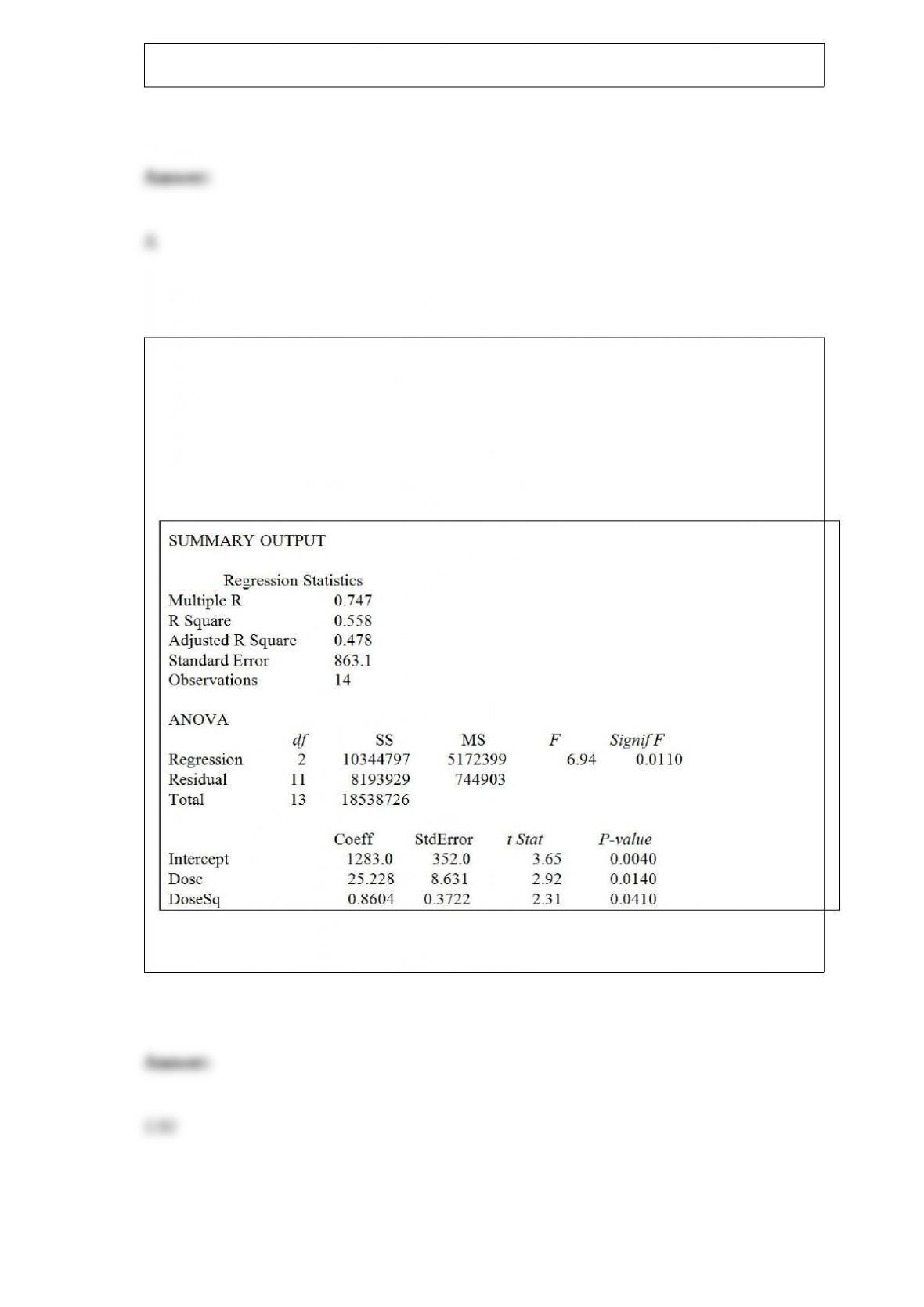
TABLE 15-3
A chemist employed by a pharmaceutical firm has developed a muscle relaxant. She
took a sample of 14 people suffering from extreme muscle constriction. She gave each a
vial containing a dose (X) of the drug and recorded the time to relief (Y) measured in
seconds for each. She fit a curvilinear model to this data. The results obtained by
Microsoft Excel follow
Referring to Table 15-3, suppose the chemist decides to use a t test to determine if the
linear term is significant. The value of the test statistic is ________.

TABLE 1-1
The manager of the customer service division of a major consumer electronics company
is interested in determining whether the customers who have purchased a Blu-ray
player made by the company over the past 12 months are satisfied with their products.
Referring to Table 1-1, the possible responses to the question “How many Blu-ray
players made by other manufacturers have you used?” result in
A) a nominal scale variable.
B) an ordinal scale variable.
C) an interval scale variable.
D) a ratio scale variable.
An economist is interested in studying the incomes of consumers in a particular country.
The population standard deviation is known to be $1,000. A random sample of 50
individuals resulted in a mean income of $15,000. What is the width of the 90%
confidence interval?
A) $232.60
B) $364.30
C) $465.23
D) $728.60

The sample correlation coefficient between X and Y is 0.375. It has been found out that
the p-value is 0.256 when testing H0 : = 0 against the one-sided alternative H1 : > 0.
To test H0 : = 0 against the two-sided alternative H1 : 0 at a significance level of
0.1, the p-value is
A) 0.256 / 2.
B) (0.256)(2).
C) 1 – 0.256.
D) 1 – 0.256 / 2.
The owner of a fish market has an assistant who has determined that the weights of
catfish are normally distributed, with a mean of 3.2 pounds and a standard deviation of
0.8 pound. If a sample of 64 fish yields a mean of 3.4 pounds, what is probability of
obtaining a sample mean this large or larger?
A) 0.0001
B) 0.0013
C) 0.0228
D) 0.4987
Suppose Z has a standard normal distribution with a mean of 0 and standard deviation
of 1. The probability that Z is more than 0.77 is ________.
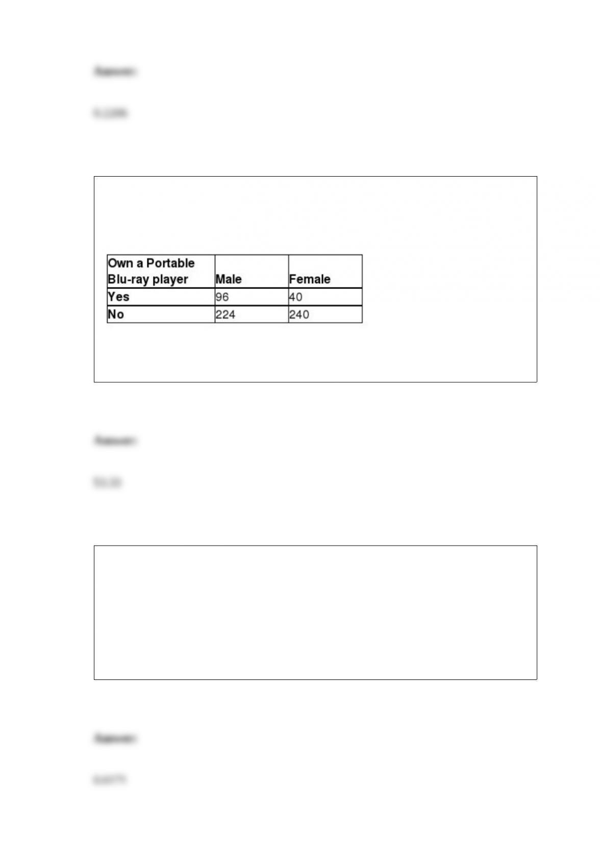
TABLE 2-14
The table below contains the number of people who own a portable Blu-ray player in a
sample of 600 broken down by gender.
Referring to Table 2-14, if the sample is a good representation of the population, we can
expect ________ percent of the population will be males.
TABLE 5-9
A major hotel chain keeps a record of the number of mishandled bags per 1,000
customers. In a recent year, the hotel chain had 4.06 mishandled bags per 1,000
customers. Assume that the number of mishandled bags has a Poisson distribution.
Referring to Table 5-9, what is the probability that in the next 1,000 customers, the
hotel chain will have no more than four mishandled bags?
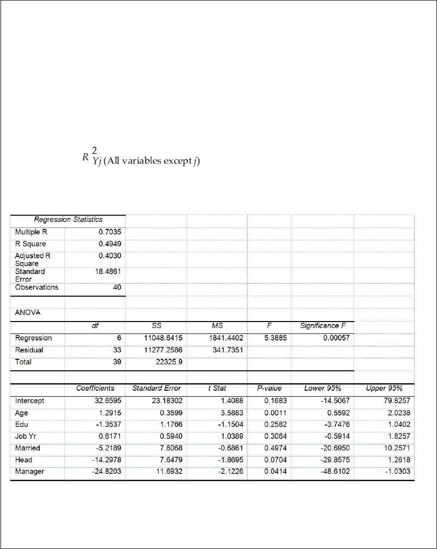
TABLE 17-10
Given below are results from the regression analysis where the dependent variable is
the number of weeks a worker is unemployed due to a layoff (Unemploy) and the
independent variables are the age of the worker (Age), the number of years of education
received (Edu), the number of years at the previous job (Job Yr), a dummy variable for
marital status (Married: 1 = married, 0 = otherwise), a dummy variable for head of
household (Head: 1 = yes, 0 = no) and a dummy variable for management position
(Manager: 1 = yes, 0 = no). We shall call this Model 1. The coefficient of partial
determination ( ) of each of the 6 predictors are, respectively,
0.2807, 0.0386, 0.0317, 0.0141, 0.0958, and 0.1201.
Model 2 is the regression analysis where the dependent variable is Unemploy and the
independent variables are Age and Manager. The results of the regression analysis are
given below:
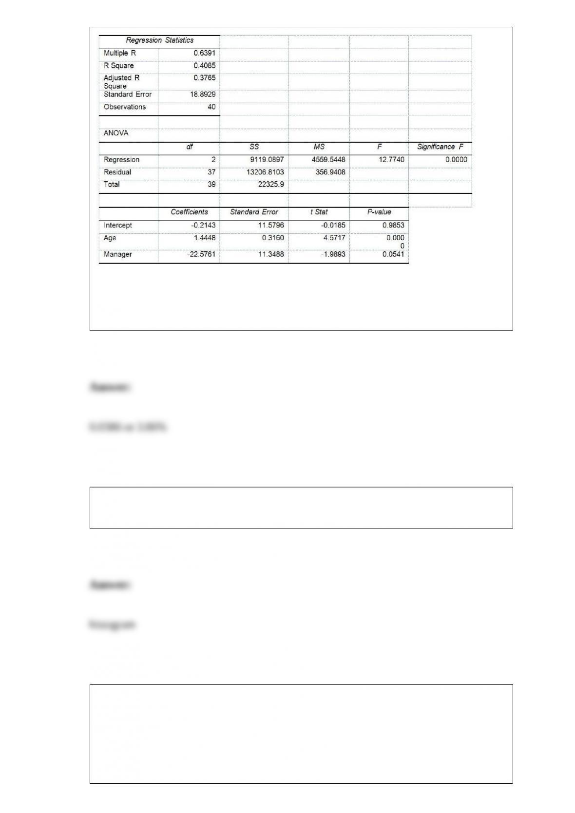
Referring to Table 17-10, Model 1, ________ of the variation in the number of weeks a
worker is unemployed due to a layoff can be explained by the number of years of
education received while controlling for the other independent variables.
A ________ is a vertical bar chart in which the rectangular bars are constructed at the
boundaries of each class interval.
TABLE 8-8
The president of a university would like to estimate the proportion of the student
population that owns a personal computer. In a sample of 500 students, 417 own a
personal computer.
Referring to Table 8-8, a 99% confidence interval for the proportion of the student
population who own a personal computer is from ________ to ________.
The amount of time required for an oil and filter change on an automobile is normally
distributed with a mean of 45 minutes and a standard deviation of 10 minutes. A
random sample of 16 cars is selected. What is the probability that the sample mean will
be between 39 and 48 minutes?
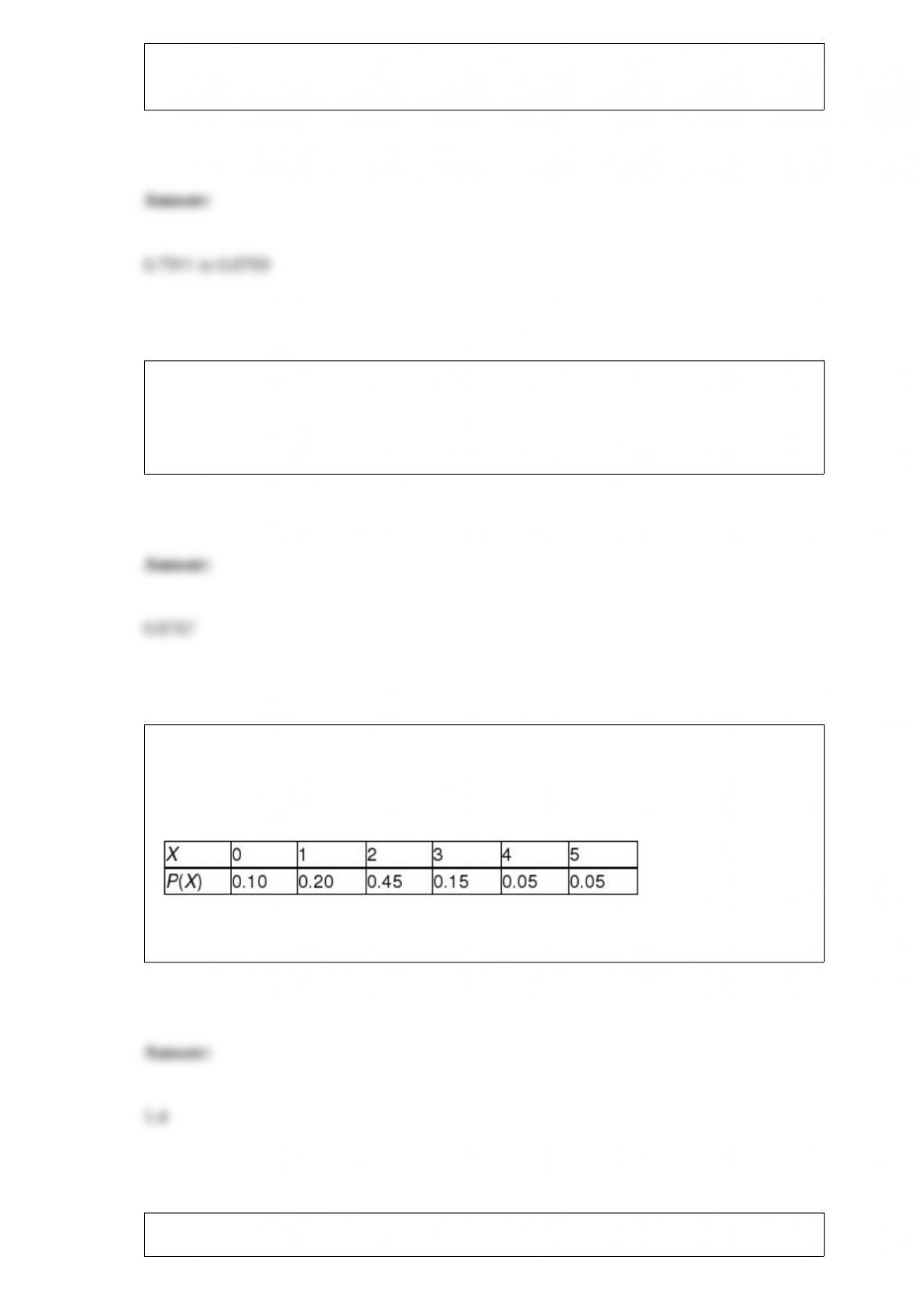
TABLE 5-4
The following table contains the probability distribution for X = the number of traffic
accidents reported in a day in Corvallis, Oregon.
Referring to Table 5-4, the variance of the number of accidents is ________.
TABLE 6-7

A company has 125 personal computers. The probability that any one of them will
require repair on a given day is 0.15.
Referring to Table 6-7 and assuming that the number of computers that requires repair
on a given day follows a binomial distribution, compute the probability that there will
be no more than 8 computers that require repair on a given day using a normal
approximation.