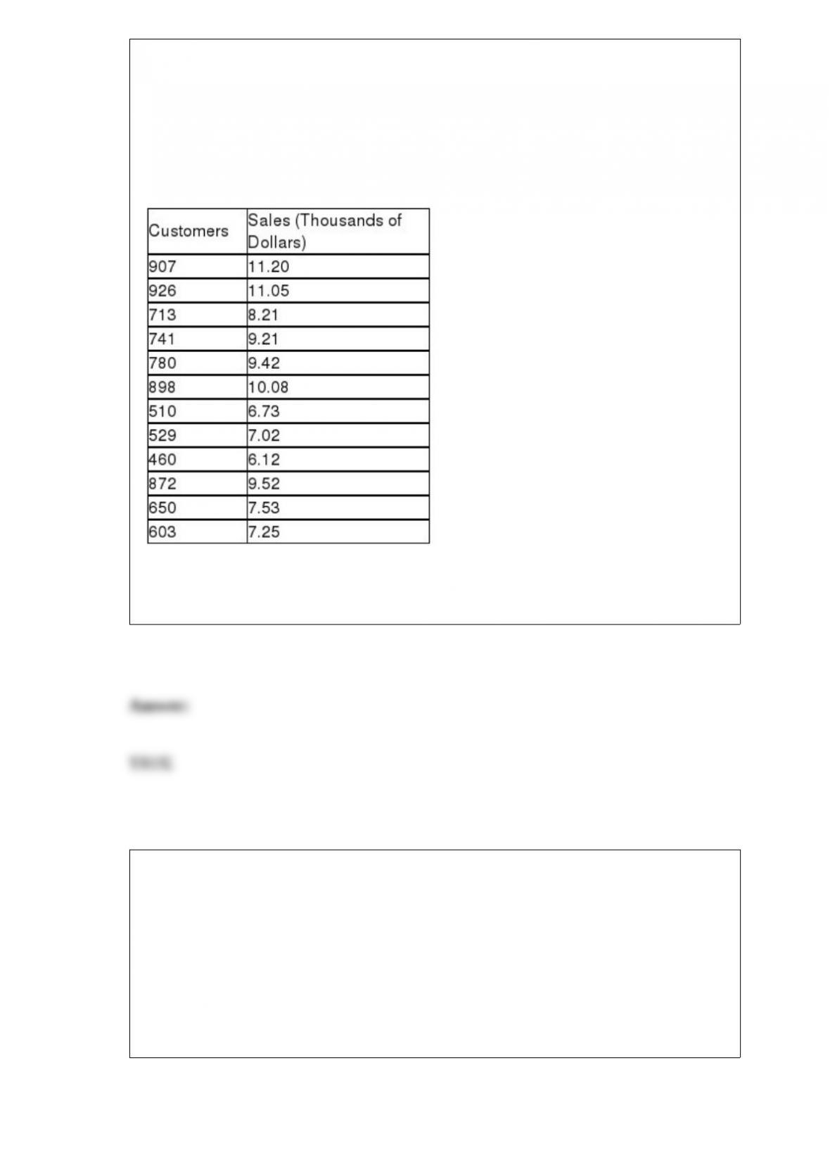
TABLE 13-10
The management of a chain electronic store would like to develop a model for
predicting the weekly sales (in thousands of dollars) for individual stores based on the
number of customers who made purchases. A random sample of 12 stores yields the
following results:
True or False: Referring to Table 13-10, it is inappropriate to compute the
Durbin-Watson statistic and test for autocorrelation in this case.
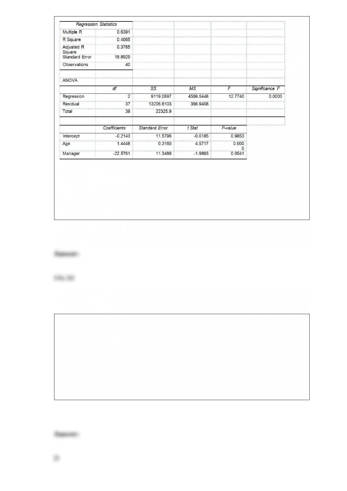
TABLE 14-17
Given below are results from the regression analysis where the
dependent variable is the number of weeks a worker is unemployed
due to a layo! (Unemploy) and the independent variables are the age
of the worker (Age) and a dummy variable for management position
(Manager: 1 = yes, 0 = no).
The results of the regression analysis are given below:

True or False: Referring to Table 14-17, the alternative hypothesis H1 :
At least one of βj ≠0 for j = 1, 2 implies that the number of weeks
a worker is unemployed due to a layo! is a!ected by all of the
explanatory variables.
TABLE 9-3
An appliance manufacturer claims to have developed a compact microwave oven that
consumes a mean of no more than 250 W. From previous studies, it is believed that
power consumption for microwave ovens is normally distributed with a population
standard deviation of 15 W. A consumer group has decided to try to discover if the
claim appears true. They take a sample of 20 microwave ovens and find that they
consume a mean of 257.3 W.
True or False: Referring to Table 9-3, the null hypothesis will be rejected at 1% level of
significance.

True or False: The level of satisfaction (“Very unsatisfied,” “Fairly unsatisfied,” “Fairly
satisfied,” and “Very satisfied”) in a class is an example of an ordinal scaled variable.
TABLE 8-6
After an extensive advertising campaign, the manager of a company wants to estimate
the proportion of potential customers that recognize a new product. She samples 120
potential consumers and finds that 54 recognize this product. She uses this sample
information to obtain a 95% confidence interval that goes from 0.36 to 0.54.
True or False: Referring to Table 8-6, it is possible that the true proportion of people
that recognize the product is between 0.36 and 0.54.
True or False: The D in the DCOVA framework stands for “define.”
True or False: The Cp index measures the potential of a process, not its actual
performance.
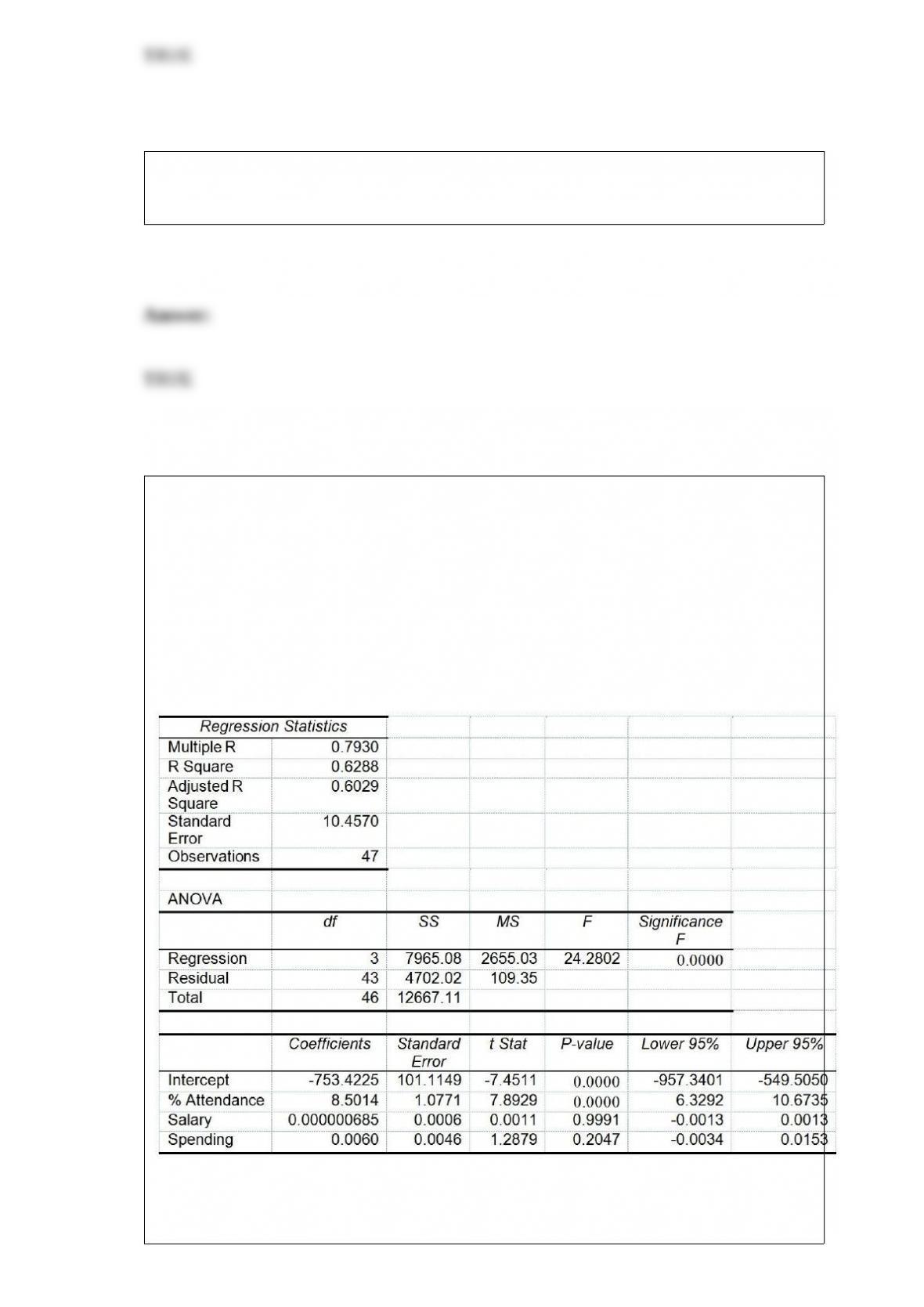
True or False: TABLE 17-8
The superintendent of a school district wanted to predict the percentage of students
passing a sixth-grade proficiency test. She obtained the data on percentage of students
passing the proficiency test (% Passing), daily mean of the percentage of students
attending class (% Attendance), mean teacher salary in dollars (Salaries), and
instructional spending per pupil in dollars (Spending) of 47 schools in the state.
Following is the multiple regression output with Y = % Passing as the dependent
variable, X1 = % Attendance, X2 = Salaries and X3 = Spending:
Referring to Table 17-8, the alternative hypothesis H1 : At least one of βj ≠0 for j =
1, 2, 3 implies that the percentage of students passing the proficiency test is related to at
least one of the explanatory variables.
True or False: Other things being equal, the confidence interval for the mean will be
wider for 95% confidence than for 90% confidence.
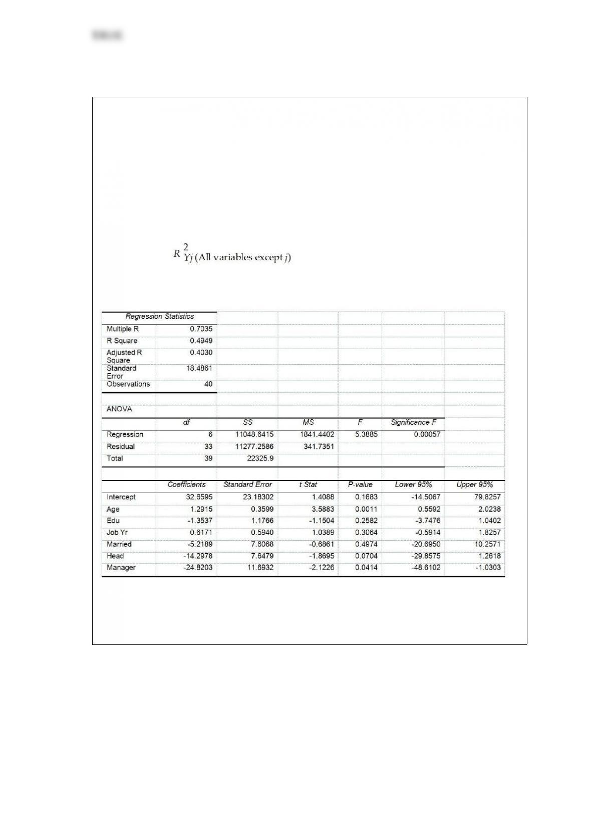
True or False: TABLE 17-10
Given below are results from the regression analysis where the dependent variable is
the number of weeks a worker is unemployed due to a layoff (Unemploy) and the
independent variables are the age of the worker (Age), the number of years of education
received (Edu), the number of years at the previous job (Job Yr), a dummy variable for
marital status (Married: 1 = married, 0 = otherwise), a dummy variable for head of
household (Head: 1 = yes, 0 = no) and a dummy variable for management position
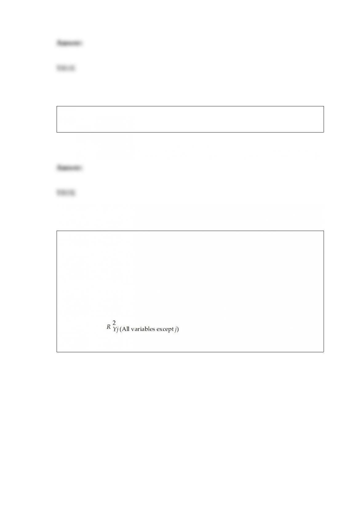
(Manager: 1 = yes, 0 = no). We shall call this Model 1. The coefficient of partial
determination ( ) of each of the 6 predictors are, respectively,
0.2807, 0.0386, 0.0317, 0.0141, 0.0958, and 0.1201.
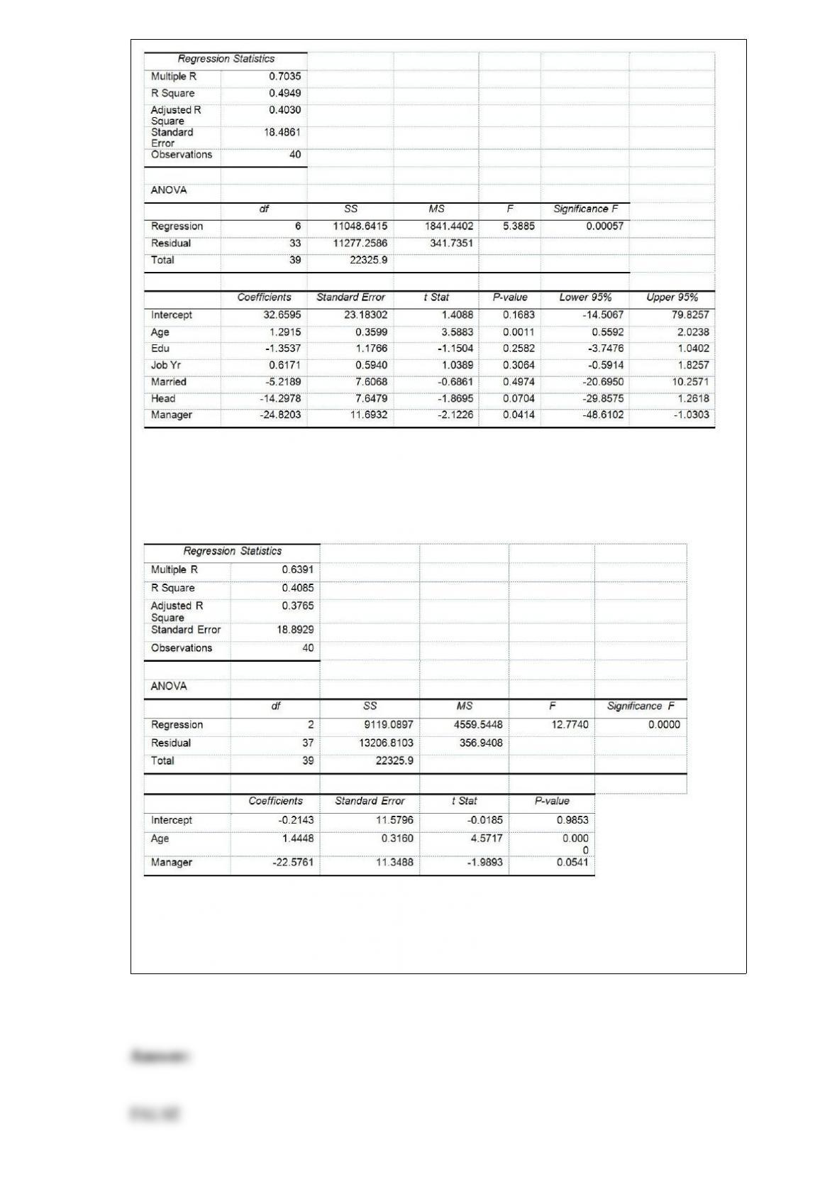
Model 2 is the regression analysis where the dependent variable is Unemploy and the
independent variables are Age and Manager. The results of the regression analysis are
given below:
Referring to Table 17-10, Model 1, there is sufficient evidence that all of the
explanatory variables are related to the number of weeks a worker is unemployed due to
a layoff at a 10% level of significance.

True or False: Referring to Table 14-7, the department head wants to
use a t test to test for the signiticance of the coefficient of X1. At a
level of signiticance of 0.05, the department head would decide that
β1 ≠0.
TABLE 14-7
The department head of the accounting department wanted to see if
she could predict the GPA of students using the number of course
units (credits) and total SAT scores of each. She takes a sample of
students and generates the following Microsoft Excel output:
True or False: TABLE 17-9
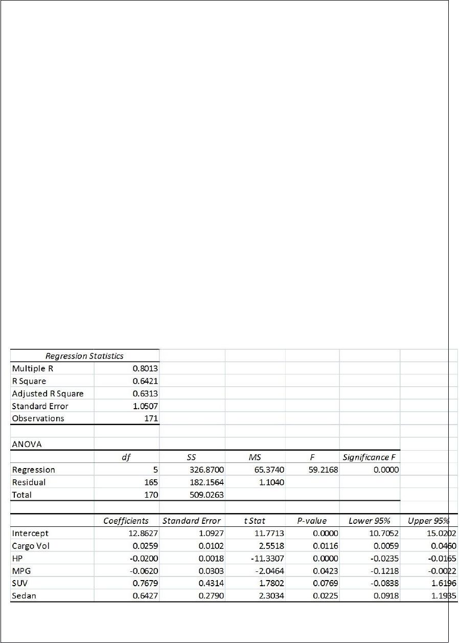
What are the factors that determine the acceleration time (in sec.) from 0 to 60 miles per
hour of a car? Data on the following variables for 171 different vehicle models were
collected:
Accel Time: Acceleration time in sec.
Cargo Vol: Cargo volume in cu. ft.
HP: Horsepower
MPG: Miles per gallon
SUV: 1 if the vehicle model is an SUV with Coupe as the base when SUV and Sedan
are both 0
Sedan: 1 if the vehicle model is a sedan with Coupe as the base when SUV and Sedan
are both 0
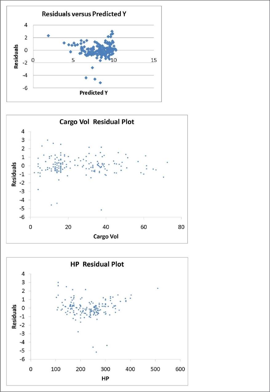
The regression results using acceleration time as the dependent variable and the
remaining variables as the independent variables are presented below.
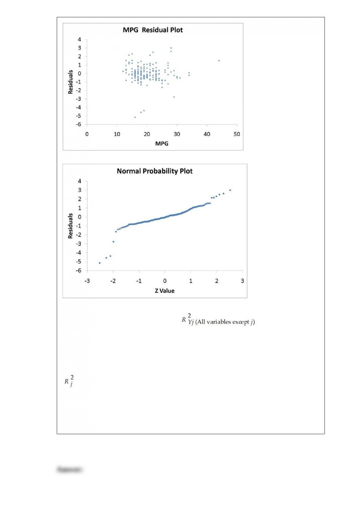
The various residual plots are as shown below.
The coefficient of partial determination ( ) of each of the 5
predictors are, respectively, 0.0380, 0.4376, 0.0248, 0.0188, and 0.0312.
The coefficient of multiple determination for the regression model using each of the 5
variables Xj as the dependent variable and all other X variables as independent variables
( ) are, respectively, 0.7461, 0.5676, 0.6764, 0.8582, 0.6632.
Referring to Table 17-9, there is enough evidence to conclude that HP makes a
significant contribution to the regression model in the presence of the other independent
variables at a 5% level of significance.
True or False: TABLE 17-10
Given below are results from the regression analysis where the dependent variable is
the number of weeks a worker is unemployed due to a layoff (Unemploy) and the
independent variables are the age of the worker (Age), the number of years of education
received (Edu), the number of years at the previous job (Job Yr), a dummy variable for
marital status (Married: 1 = married, 0 = otherwise), a dummy variable for head of
household (Head: 1 = yes, 0 = no) and a dummy variable for management position
(Manager: 1 = yes, 0 = no). We shall call this Model 1. The coefficient of partial
determination ( ) of each of the 6 predictors are, respectively,
0.2807, 0.0386, 0.0317, 0.0141, 0.0958, and 0.1201.
Model 2 is the regression analysis where the dependent variable is Unemploy and the
independent variables are Age and Manager. The results of the regression analysis are
given below:
Referring to Table 17-10, Model 1, we can conclude that, holding constant the effect of
the other independent variables, there is a difference in the mean number of weeks a
worker is unemployed due to a layoff between a worker who is married and one who is
not at a 5% level of significance if we use only the information of the 95% confidence
interval estimate for β4.
When would you use the Tukey-Kramer procedure?
A) to test for normality
B) to test for homogeneity of variance
C) to test independence of errors
D) to test for differences in pairs of means
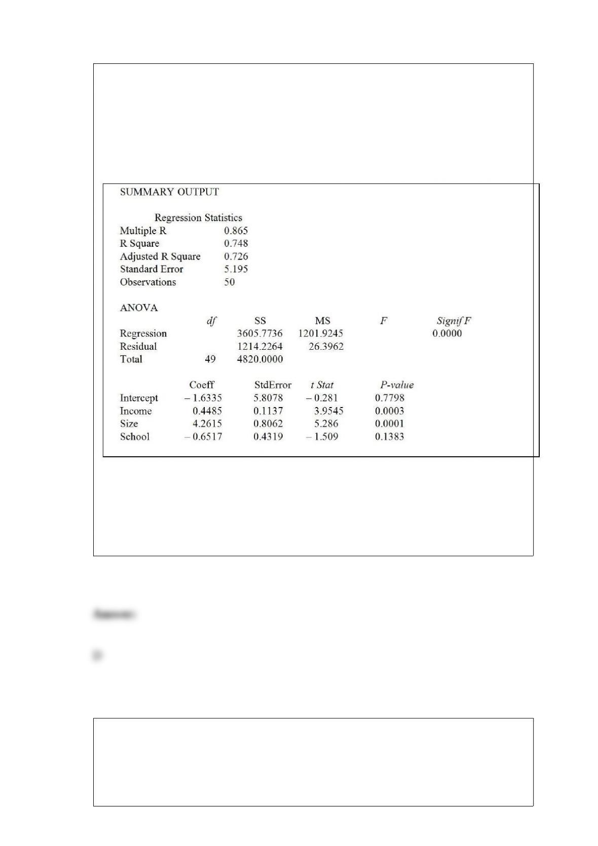
TABLE 17-1
A real estate builder wishes to determine how house size (House) is influenced by
family income (Income), family size (Size), and education of the head of household
(School). House size is measured in hundreds of square feet, income is measured in
thousands of dollars, and education is in years. The builder randomly selected 50
families and ran the multiple regression. Microsoft Excel output is provided below:
Referring to Table 17-1, suppose the builder wants to test whether the coefficient on
School is significantly different from 0. What is the value of the relevant t-statistic?
A) 5.286
B) 5.195
C) 3.945
D) -1.509
Jared was working on a project to look at global warming and accessed an Internet site
where he captured average global surface temperatures from 1866. Which of the four
methods of data collection was he using?
A) published sources
B) experimentation
C) surveying
D) observation
TABLE 10-3
A real estate company is interested in testing whether the mean time that families in
Gotham have been living in their current homes is less than families in Metropolis.
Assume that the two population variances are equal. A random sample of 100 families
from Gotham and a random sample of 150 families in Metropolis yield the following
data on length of residence in current homes.
Gotham: G = 35 months, = 900 Metropolis: M = 50 months, = 1050
Referring to Table 10-3, suppose = 0.10. Which of the following represents the correct
conclusion?
A) There is not enough evidence that the mean amount of time families in Gotham have
been living in their current homes is less than families in Metropolis.
B) There is enough evidence that the mean amount of time families in Gotham have
been living in their current homes is less than families in Metropolis.
C) There is not enough evidence that the mean amount of time families in Gotham have
been living in their current homes is not less than families in Metropolis.
D) There is enough evidence that the mean amount of time families in Gotham have
been living in their current homes is not less than families in Metropolis.

Referring to Table 14-15, which of the following is a correct
statement?
TABLE 14-15
The superintendent of a school district wanted to predict the
percentage of students passing a sixth-grade proficiency test. She
obtained the data on percentage of students passing the proficiency
test (% Passing), mean teacher salary in thousands of dollars
(Salaries), and instructional spending per pupil in thousands of dollars
(Spending) of 47 schools in the state.
Following is the multiple regression output with Y = % Passing as the
dependent variable, X1 = Salaries and X2 = Spending:
A) The mean percentage of students passing the proficiency test is
estimated to go up by 2.79% when mean teacher salary increases by
one thousand dollars.
B) The mean teacher salary is estimated to go up by 2.79% when
mean percentage of students passing the proficiency test increases
by 1%.
C) The mean percentage of students passing the proficiency test is
estimated to go up by 2.79% when mean teacher salary increases by
one thousand dollars holding constant the instructional spending per
pupil.
D) The mean teacher salary is estimated to go up by 2.79% when
mean percentage of students passing the proficiency test increases
by 1% holding constant the instructional spending per pupil.

A sample of 300 subscribers to a particular magazine is selected from a population
frame of 9,000 subscribers. If, upon examining the data, it is determined that no
subscriber had been selected in the sample more than once,
A) the sample could not have been random.
B) the sample may have been selected without replacement or with replacement.
C) the sample had to have been selected with replacement.
D) the sample had to have been selected without replacement.
Referring to Table 14-6, what is the 95% confidence interval for the expected change in
heating costs as a result of a 1 degree Fahrenheit change in the daily minimum outside
temperature?
TABLE 14-6
One of the most common questions of prospective house buyers pertains to the cost of
heating in dollars (Y). To provide its customers with information on that matter, a large
real estate firm used the following 2 variables to predict heating costs: the daily
minimum outside temperature in degrees of Fahrenheit (X1) and the amount of
insulation in inches (X2). Given below is EXCEL output of the regression model.
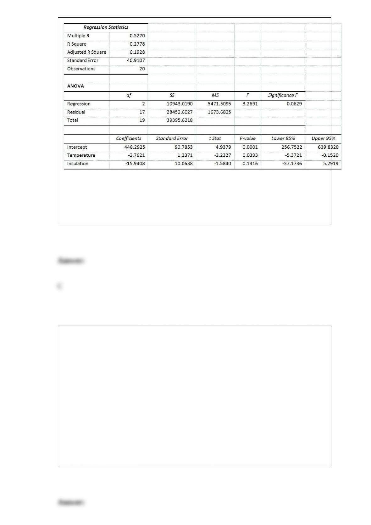
Also SSR (X1∣ X2) = 8343.3572 and SSR (X2∣ X1) = 4199.2672
A) [256.7522, 639.8328]
B) [204.7854, 497.1733]
C) [-5.3721, -0.1520]
D) [-37.1736, 5.2919]
Referring to Table 14-16, what is the correct interpretation for the estimated coefficient
for X2?
A) The mean 0 to 60 miles per hour acceleration time of a sedan is estimated to be
0.7264 seconds lower than that of a non-sedan after considering the effect of the engine
size.
B) The mean 0 to 60 miles per hour acceleration time of a sedan is estimated to be
0.7264 seconds higher than that of a non-sedan after considering the effect of the engine
size.
C) The mean 0 to 60 miles per hour acceleration time of a sedan is estimated to be
0.7264 seconds lower than that of a non-sedan without considering the effect of the
engine size.
D) The mean 0 to 60 miles per hour acceleration time of a sedan is estimated to be
0.7264 seconds higher than that of a non-sedan without considering the effect of the
engine size.
TABLE 17-4
You decide to predict gasoline prices in different cities and towns in the United States
for your term project. Your dependent variable is price of gasoline per gallon and your
explanatory variables are per capita income, the number of firms that manufacture
automobile parts in and around the city, the number of new business starts in the last
year, population density of the city, percentage of local taxes on gasoline, and the
number of people using public transportation. You collected data of 32 cities and
obtained a regression sum of squares SSR= 122.8821. Your computed value of standard
error of the estimate is 1.9549.
Referring to Table 17-4, what is the value of the coefficient of multiple determination?
A) 0.2225
B) 0.4576
C) 0.5626
D) 0.6472
The control chart
A) focuses on the time dimension of a system.
B) captures the natural variability in the system.
C) can be used for categorical, discrete, or continuous variables.
D) All of the above.
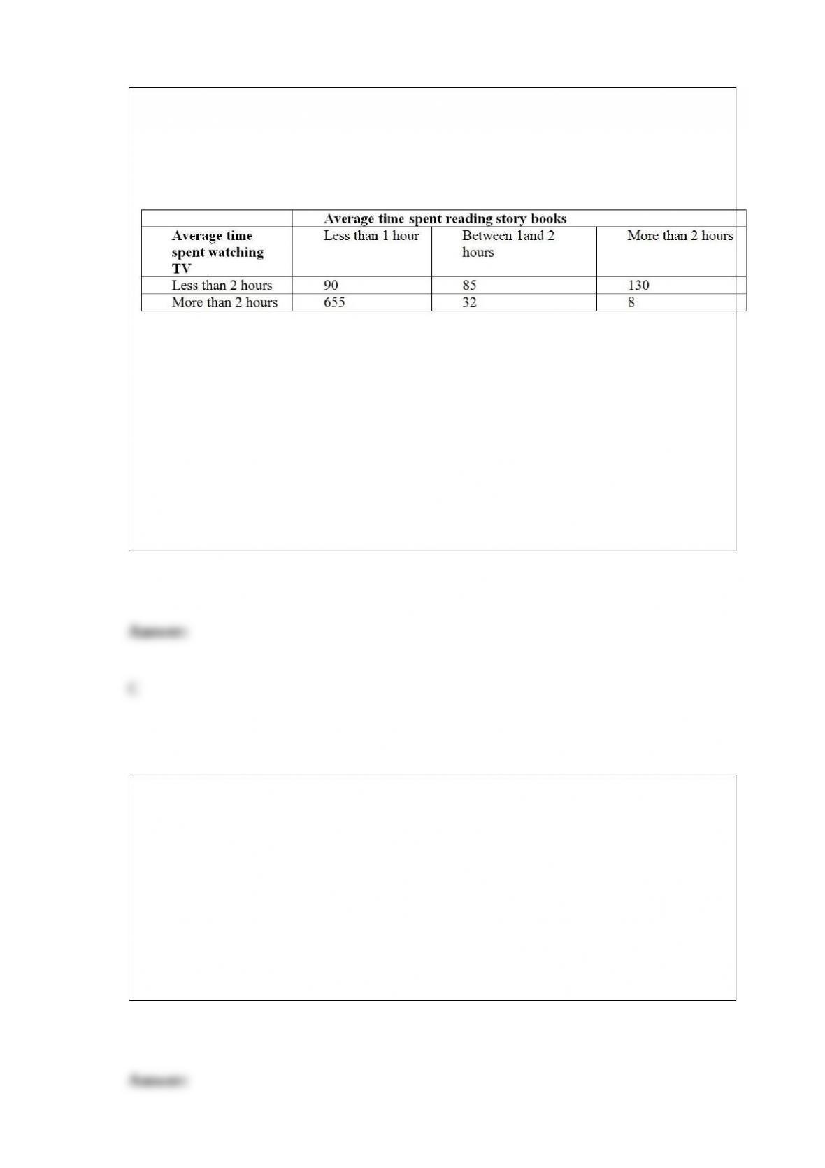
TABLE 12-12
Parents complain that children read too few storybooks and watch too much television
nowadays. A survey of 1,000 children reveals the following information on average
time spent watching TV and average time spent reading storybooks.
Referring to Table 12-12, how many children in the survey spent less than 2 hours
watching TV and no more than 2 hours reading storybooks on average?
A) 8
B) 130
C) 175
D) 687
For a population frame containing N = 1,007 individuals, what code number should you
assign to the first person on the list in order to use a table of random numbers?
A) 0
B) 1
C) 01
D) 0001

The amount of tea leaves in a can from a particular production line is normally
distributed with = 110 grams and = 25 grams. A sample of 25 cans is to be selected.
So, 95% of all sample means will be greater than how many grams?
TABLE 8-3
To become an actuary, it is necessary to pass a series of 10 exams, including the most
important one, an exam in probability and statistics. An insurance company wants to
estimate the mean score on this exam for actuarial students who have enrolled in a
special study program. They take a sample of 8 actuarial students in this program and
determine that their scores are: 2, 5, 8, 8, 7, 6, 5, and 7. This sample will be used to
calculate a 90% confidence interval for the mean score for actuarial students in the
special study program.
Referring to Table 8-3, the confidence interval will be based on ________ degrees of
freedom.
TABLE 12-6
According to an article in Marketing News, fewer checks are being written at the
grocery store checkout than in the past. To determine whether there is a difference in
the proportion of shoppers who pay by check among three consecutive years at a 0.05
level of significance, the results of a survey of 500 shoppers in three consecutive years
are obtained and presented below.
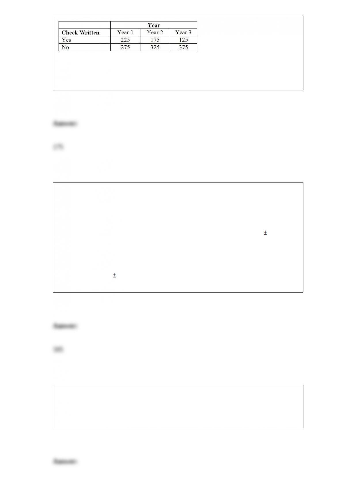
Referring to Table 12-6, what is the expected number of shoppers who pay by check in
year 1 if there is no difference in the proportion of shoppers who pay by check among
the three years?
TABLE 8-11
A poll was conducted by the marketing department of a video game company to
determine the popularity of a new game that was targeted to be launched in three
months. Telephone interviews with 1,500 young adults were conducted which revealed
that 49% said they would purchase the new game. The margin of error was 3
percentage points.
Referring to Table 8-11, what is the needed sample size to obtain a 95% confidence
interval in estimating the percentage of the targeted young adults who will purchase the
new game to within 5% if you do not have the information on the 49% in the
interviews who said that they would purchase the new game?
Microsoft Excel was used to obtain the following quadratic trend equation:
Sales = 100 – 10X + 15X2.
The data used was from 2001 through 2010 coded 0 to 9. The forecast for 2011 is
________.
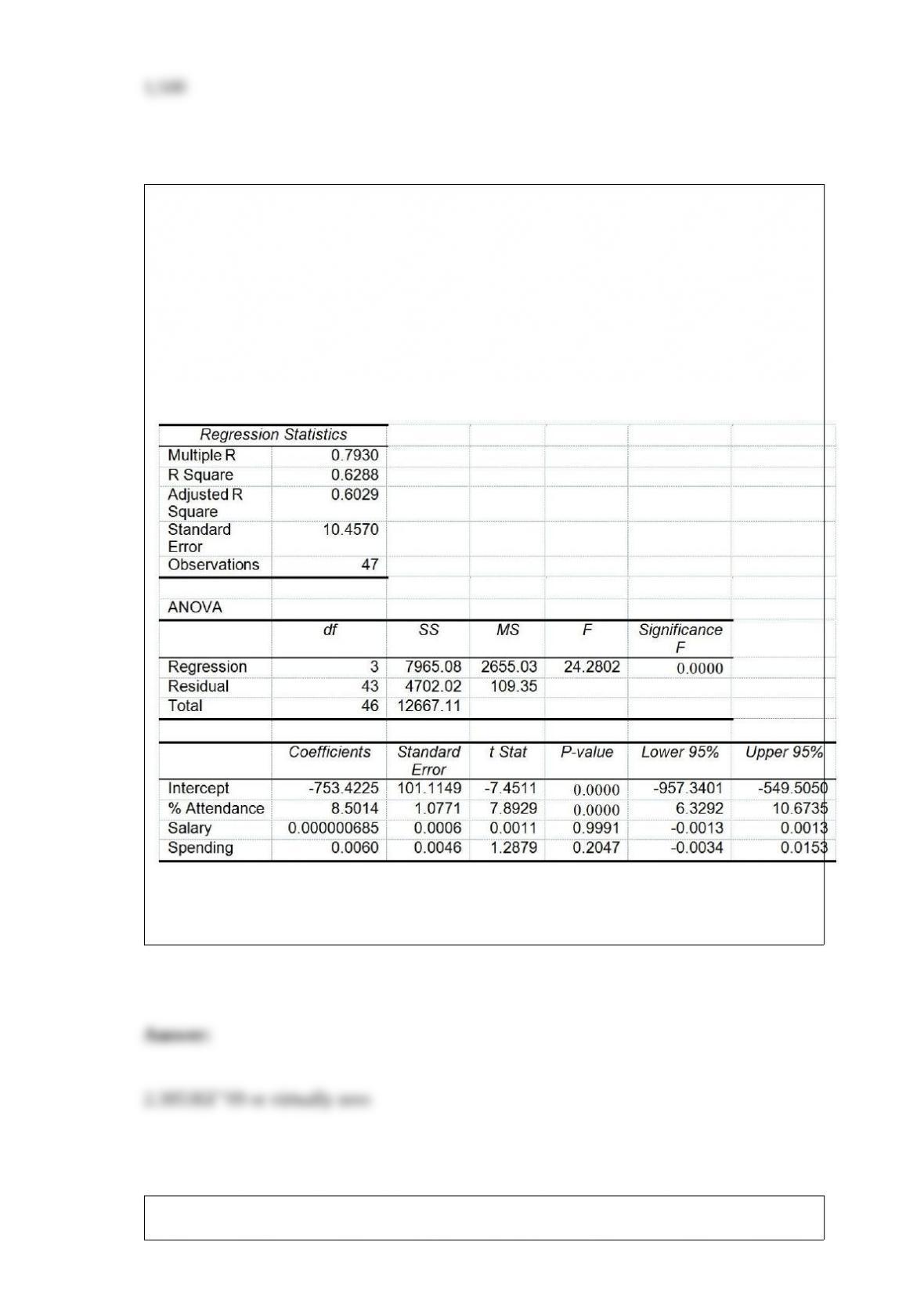
TABLE 17-8
The superintendent of a school district wanted to predict the percentage of students
passing a sixth-grade proficiency test. She obtained the data on percentage of students
passing the proficiency test (% Passing), daily mean of the percentage of students
attending class (% Attendance), mean teacher salary in dollars (Salaries), and
instructional spending per pupil in dollars (Spending) of 47 schools in the state.
Following is the multiple regression output with Y = % Passing as the dependent
variable, X1 = % Attendance, X2 = Salaries and X3 = Spending:
Referring to Table 17-8, what is the p-value of the test statistic to determine whether
there is a significant relationship between the percentage of students passing the
proficiency test and the entire set of explanatory variables?
Referring to Table 14-19, what is the estimated odds ratio for a home

owner with a family income of $100,000 and a lawn size of 2,000
square feet?
TABLE 14-19
The marketing manager for a nationally franchised lawn service
company would like to study the characteristics that di!erentiate
home owners who do and do not have a lawn service. A random
sample of 30 home owners located in a suburban area near a large
city was selected; 11 did not have a lawn service (code 0) and 19 had
a lawn service (code 1). Additional information available concerning
these 30 home owners includes family income (Income, in thousands
of dollars) and lawn size (Lawn Size, in thousands of square feet).
The PHStat output is given below:
TABLE 7-4
According to a survey, only 15% of customers who visited the website of a major retail
store made a purchase. Random sample sizes of 50 are selected.
Referring to Table 7-4, what is the probability that a random sample of 50 will have at
least 30% of customers who will make a purchase after visiting the website?