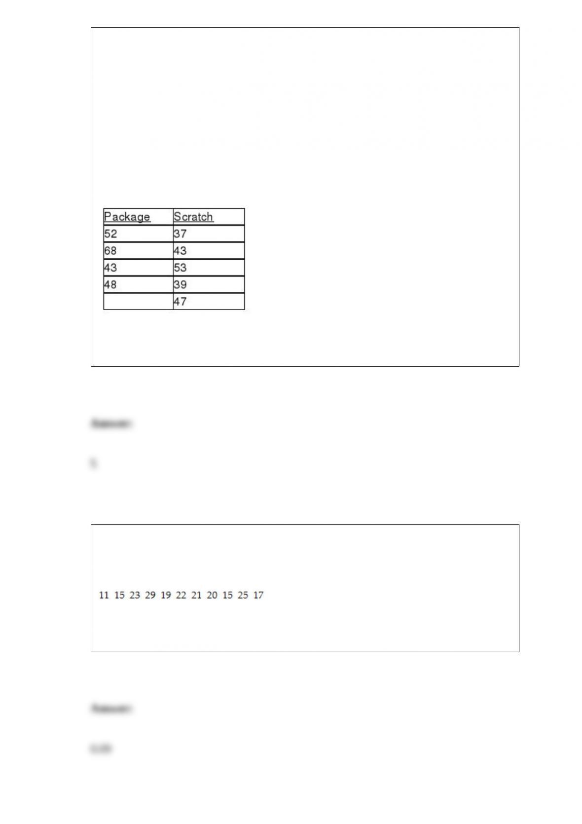
TABLE 12-14
A perfume manufacturer is trying to choose between 2 magazine advertising layouts.
An expensive layout would include a small package of the perfume. A cheaper layout
would include a ‘scratch-and-sniff” sample of the product. The manufacturer would use
the more expensive layout only if there is evidence that it would lead to a higher
approval rate. The manufacturer presents the more expensive layout to 4 groups and
determines the approval rating for each group. He presents the ‘scratch-and-sniff” layout
to 5 groups and again determines the approval rating of the perfume for each group. The
data are given below. Use this to test the appropriate hypotheses with the Wilcoxon
Rank Sum Test with a level of significance of 0.05.
Referring to Table 12-14, the rank given to the last observation in the ‘scratch-and-sniff”
group is ________.
TABLE 3-2
The data below represent the amount of grams of carbohydrates in a serving of
breakfast cereal in a sample of 11 different servings.
Referring to Table 3-2, the skewness statistic for the carbohydrate amount in the cereal
is ________.
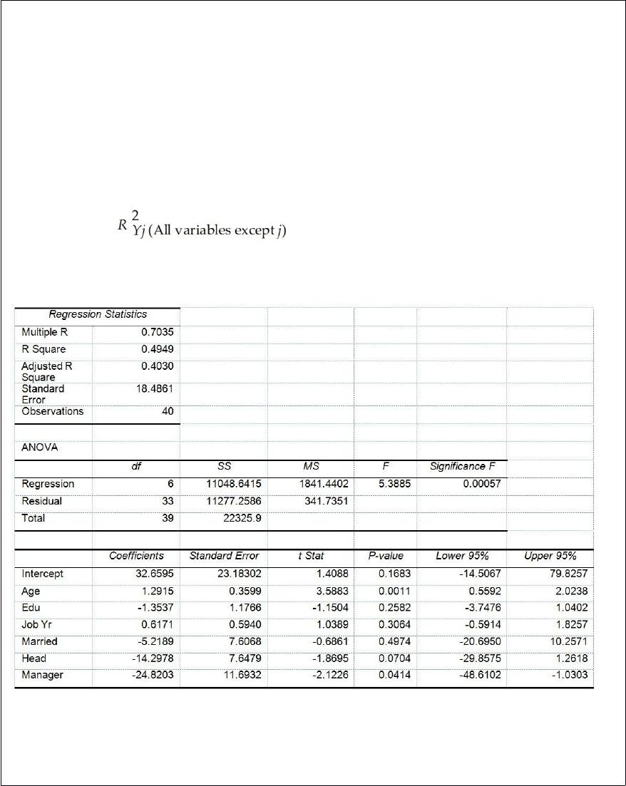
TABLE 17-10
Given below are results from the regression analysis where the dependent variable is
the number of weeks a worker is unemployed due to a layoff (Unemploy) and the
independent variables are the age of the worker (Age), the number of years of education
received (Edu), the number of years at the previous job (Job Yr), a dummy variable for
marital status (Married: 1 = married, 0 = otherwise), a dummy variable for head of
household (Head: 1 = yes, 0 = no) and a dummy variable for management position
(Manager: 1 = yes, 0 = no). We shall call this Model 1. The coefficient of partial
determination ( ) of each of the 6 predictors are, respectively,
0.2807, 0.0386, 0.0317, 0.0141, 0.0958, and 0.1201.
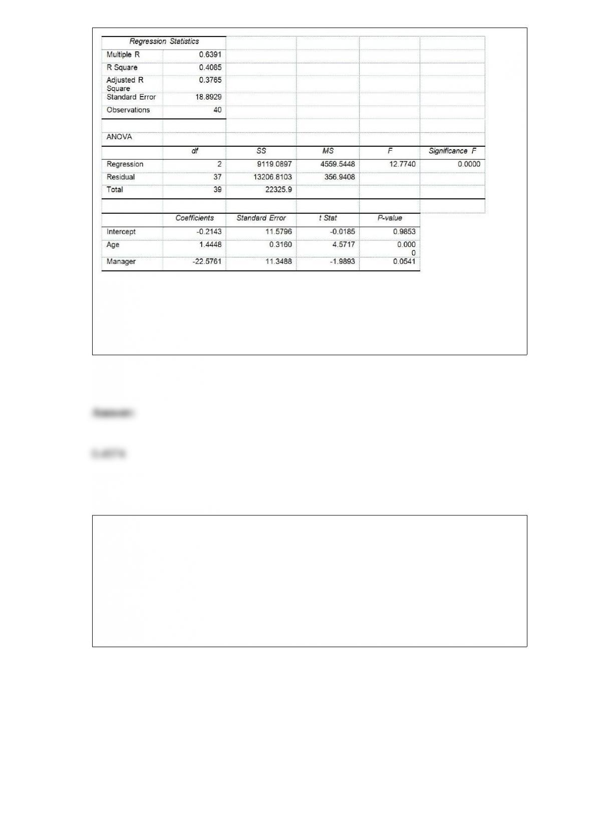
Model 2 is the regression analysis where the dependent variable is Unemploy and the
independent variables are Age and Manager. The results of the regression analysis are
given below:
Referring to Table 17-10, Model 1, what is the p-value of the test statistic when testing
whether being married or not makes a difference in the mean number of weeks a worker
is unemployed due to a layoff while holding constant the effect of all the other
independent variables?
TABLE 13-13
In this era of tough economic conditions, voters increasingly ask the question: “Is the
educational achievement level of students dependent on the amount of money the state
in which they reside spends on education?” The partial computer output below is the
result of using spending per student ($) as the independent variable and composite score
which is the sum of the math, science and reading scores as the dependent variable on
35 states that participated in a study. The table includes only partial results.
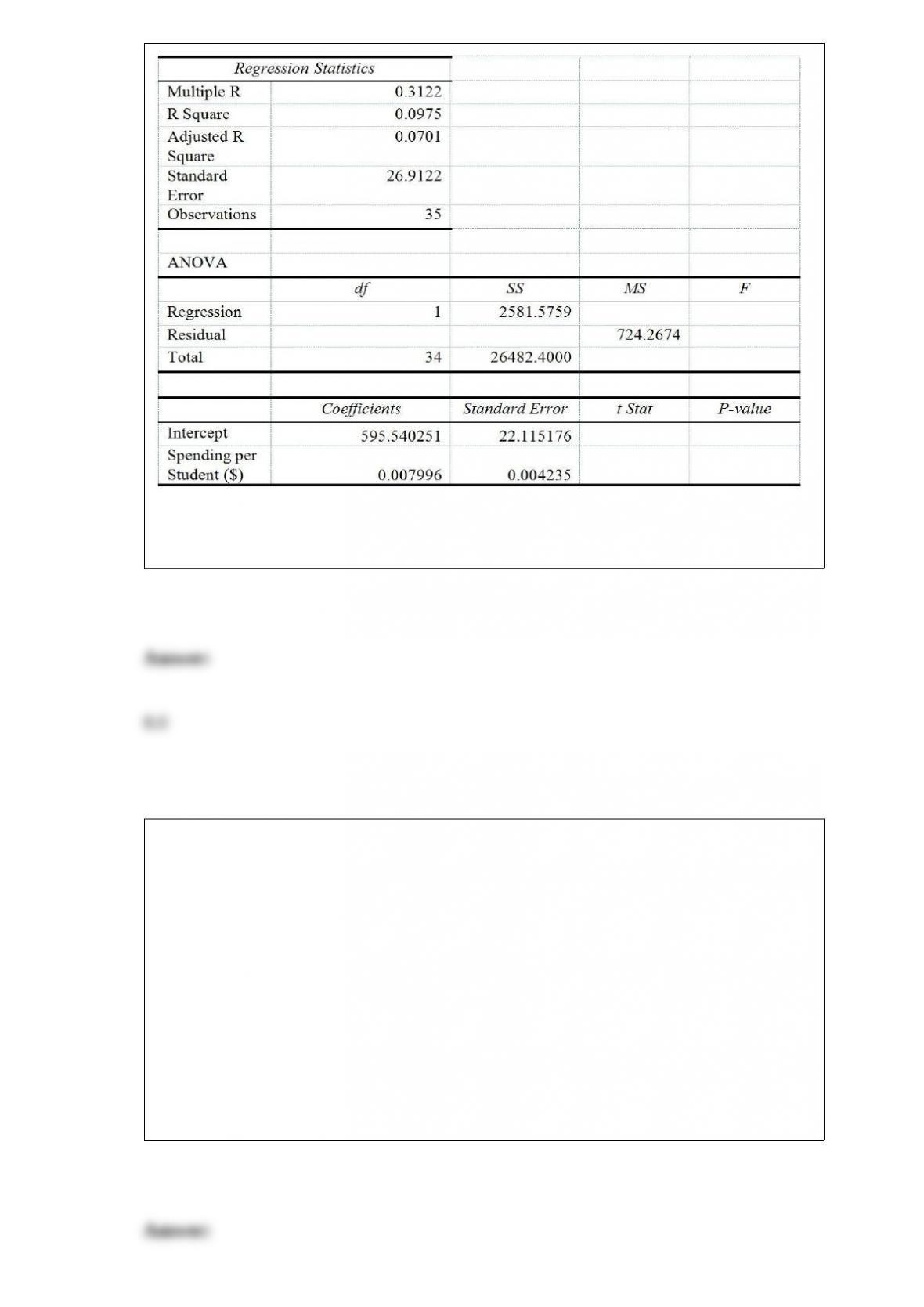
Referring to Table 13-13, if the state decides to spend 1,000 dollars more per student,
the estimated change in mean composite score is ________.
TABLE 8-13
A wealthy real estate investor wants to decide whether it is a good investment to build a
high-end shopping complex in a suburban county in Houston. His main concern is the
total market value of the 3,605 houses in the suburban county. He commissioned a
statistical consulting group to take a sample of 200 houses and obtained a sample mean
market price of $225,000 and a sample standard deviation of $38,700. The consulting
group also found out that the mean differences between market prices and appraised
prices was $125,000 with a standard deviation of $3,400. Also the proportion of houses
in the sample that are appraised for higher than the market prices is 0.24.
Referring to Table 8-13, what will be the 90% confidence interval for the population
proportion of houses that will be appraised for higher than the market prices?

TABLE 6-6
According to Investment Digest, the arithmetic mean of the annual return for common
stocks over an 85-year period was 9.5%, but the value of the variance was not
mentioned. Also 25% of the annual returns were below 8%, while 65% of the annual
returns were between 8% and 11.5%. The article claimed that the distribution of annual
return for common stocks was bell-shaped and approximately symmetric. Assume that
this distribution is normal with the mean given above. Answer the following questions
without the help of a calculator, statistical software or statistical table.
Referring to Table 6-6, 75% of the annual returns will be lower than what value?
TABLE 13-5
The managing partner of an advertising agency believes that his company’s sales are
related to the industry sales. He uses Microsoft Excel to analyze the last 4 years of
quarterly data (i.e., n = 16) with the following results:
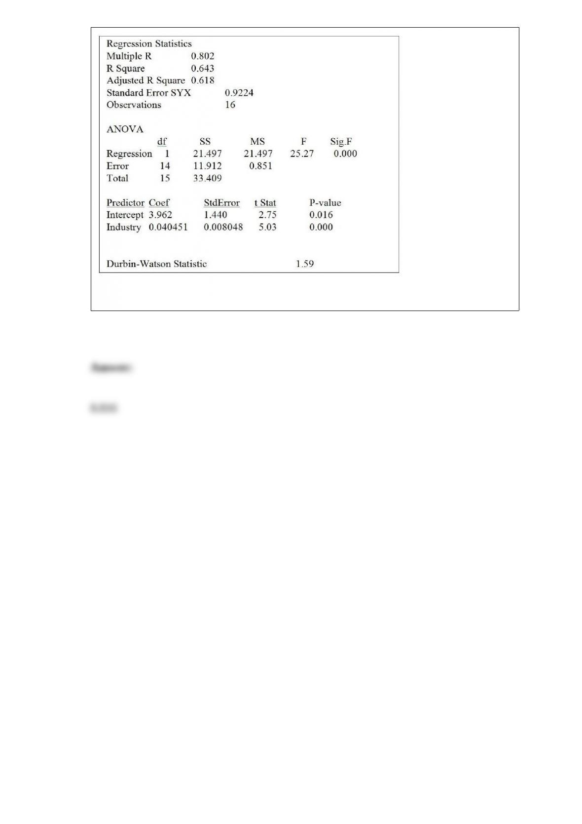
Referring to Table 13-5, the prediction for a quarter in which X = 120 is Y = ________.