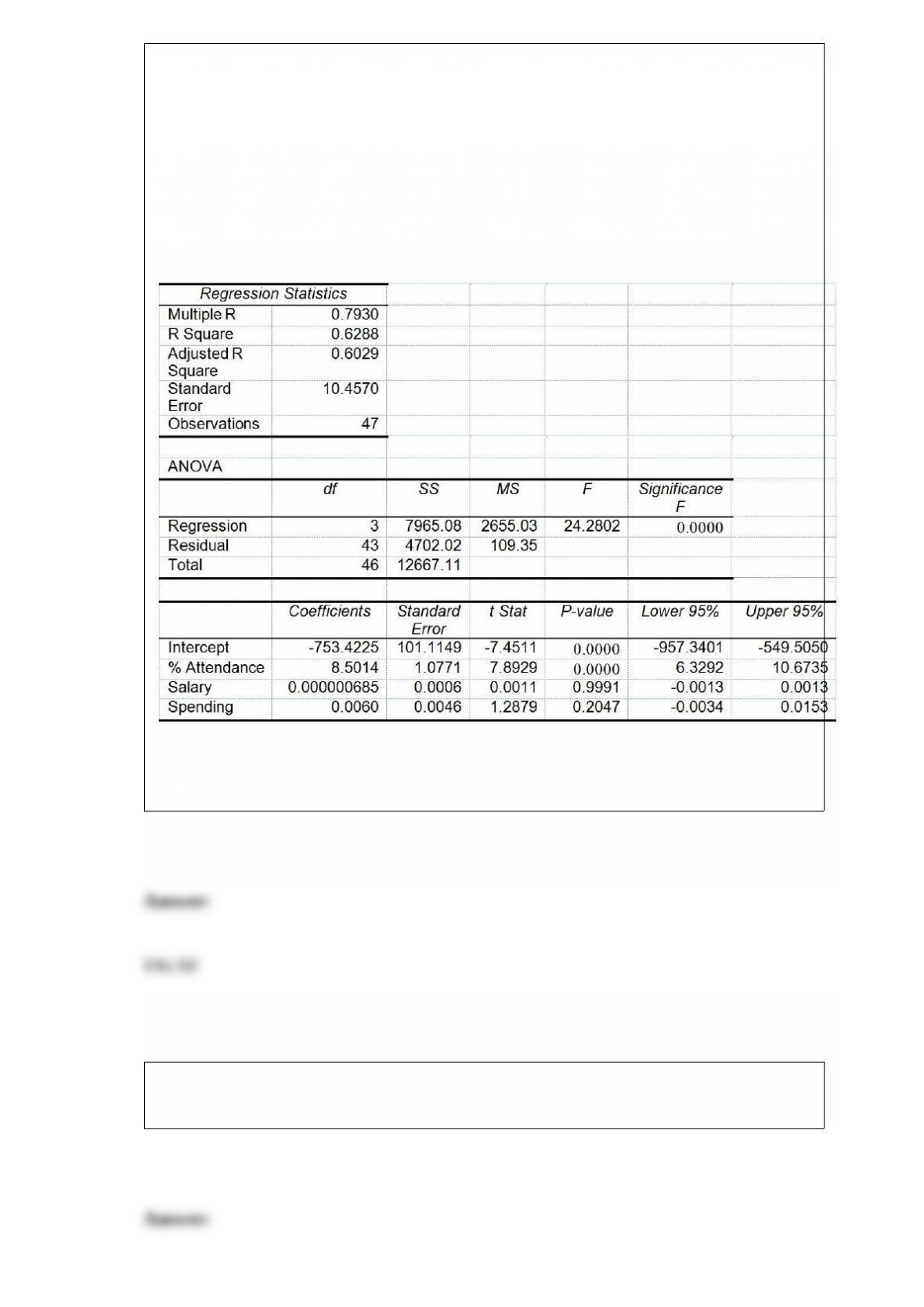
True or False: TABLE 17-8
The superintendent of a school district wanted to predict the percentage of students
passing a sixth-grade proficiency test. She obtained the data on percentage of students
passing the proficiency test (% Passing), daily mean of the percentage of students
attending class (% Attendance), mean teacher salary in dollars (Salaries), and
instructional spending per pupil in dollars (Spending) of 47 schools in the state.
Following is the multiple regression output with Y = % Passing as the dependent
variable, X1 = % Attendance, X2 = Salaries and X3 = Spending:
Referring to Table 17-8, the null hypothesis H0 : β1 = β2 = β3 = 0 implies that the
percentage of students passing the proficiency test is not related to one of the
explanatory variables.
True or False: In stepwise regression, an independent variable is not allowed to be
removed from the model once it has entered into the model.

True or False: The number of defective apples in a single box is an example of a
continuous variable.
TABLE 9-9
The president of a university claimed that the entering class this year appeared to be
larger than the entering class from previous years but their mean SAT score is lower
than previous years. He took a sample of 20 of this year’s entering students and found
that their mean SAT score is 1,501 with a standard deviation of 53. The university’s
record indicates that the mean SAT score for entering students from previous years is
1,520. He wants to find out if his claim is supported by the evidence at a 5% level of
significance.
True or False: Referring to Table 9-9, the evidence proves beyond a doubt that the mean
SAT score of the entering class this year is lower than previous years.
TABLE 8-5
A sample of salary offers (in thousands of dollars) given to management majors is: 48,
51, 46, 52, 47, 48, 47, 50, 51, and 59. Using this data to obtain a 95% confidence
interval resulted in an interval from 47.19 to 52.61.
True or False: Referring to Table 8-5, the confidence interval obtained is valid only if
the distribution of the population of salary offers is normal.

True or False: In a one-factor ANOVA analysis, the among sum of squares and within
sum of squares must add up to the total sum of squares.
True or False: A professor of economics at a small Texas university wanted to determine
what year in school students were taking his tough economics course. Data were
collected on the class status (“freshman”, ‘sophomore”, “junior” or ‘senior”) of 50
students enrolled in one of his economics course. A side-by-side bar chart can be used
to present this information.
True or False: Referring to Table 14-15, the null hypothesis should be
rejected at a 5% level of signi cance when testing whether
instructional spending per pupil has any e”ect on percentage of
students passing the pro ciency test, taking into account the e”ect of
mean teacher salary.
TABLE 14-15
The superintendent of a school district wanted to predict the
percentage of students passing a sixth-grade pro ciency test. She
obtained the data on percentage of students passing the pro ciency

test (% Passing), mean teacher salary in thousands of dollars
(Salaries), and instructional spending per pupil in thousands of dollars
(Spending) of 47 schools in the state.
Following is the multiple regression output with Y = % Passing as the
dependent variable, X1 = Salaries and X2 = Spending:
TABLE 10-5
To test the effectiveness of a business school preparation course, 8 students took a
general business test before and after the course. The results are given below.
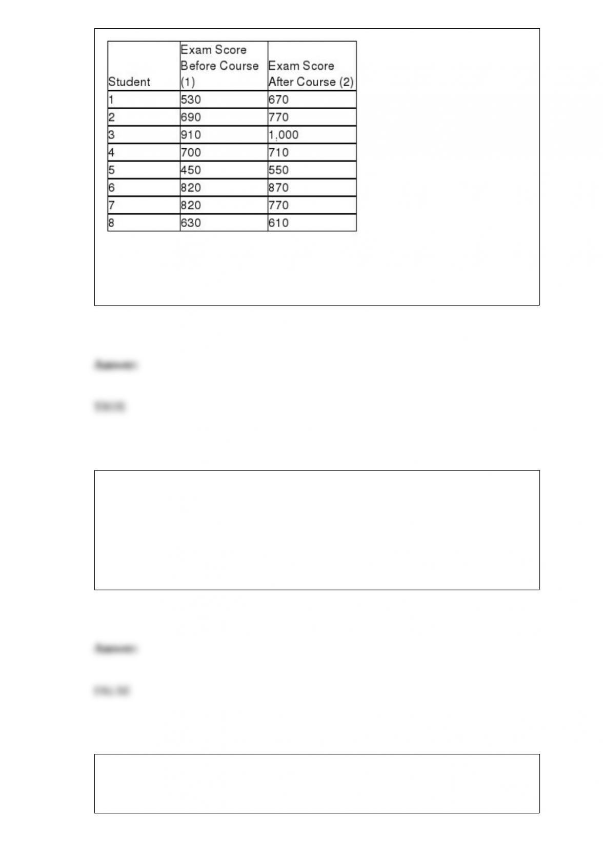
True or False: Referring to Table 10-5, in examining the differences between related
samples we are essentially sampling from an underlying population of difference
‘scores.”
TABLE 8-4
The actual voltages of power packs labeled as 12 volts are as follows: 11.77, 11.90,
11.64, 11.84, 12.13, 11.99, and 11.77.
True or False: Referring to Table 8-4, a 99% confidence interval will contain 99% of the
voltages for all such power packs.
TABLE 9-9
The president of a university claimed that the entering class this year appeared to be

larger than the entering class from previous years but their mean SAT score is lower
than previous years. He took a sample of 20 of this year’s entering students and found
that their mean SAT score is 1,501 with a standard deviation of 53. The university’s
record indicates that the mean SAT score for entering students from previous years is
1,520. He wants to find out if his claim is supported by the evidence at a 5% level of
significance.
True or False: Referring to Table 9-9, if these data were used to perform a two-tail test,
the p-value would be 0.1254.
TABLE 8-6
After an extensive advertising campaign, the manager of a company wants to estimate
the proportion of potential customers that recognize a new product. She samples 120
potential consumers and finds that 54 recognize this product. She uses this sample
information to obtain a 95% confidence interval that goes from 0.36 to 0.54.
True or False: Referring to Table 8-6, this interval requires the assumption that the
distribution of the number of people recognizing the product has a normal distribution.
TABLE 8-17
A random sample of 100 stores from a large chain of 500 garden supply stores was
selected to determine the mean number of lawnmowers sold at an end-of-season
clearance sale. The sample results indicated a mean of 6 and a standard deviation of 2
lawnmowers sold. A 95% confidence interval (5.623 to 6.377) was established based on
these results.
True or False: Referring to Table 8-17, of all possible samples of 100 stores drawn from
the population of 1,000 stores, 95% of the sample means will fall between 5.623 and
6.377 lawnmowers.
True or False: An insurance company evaluates many variables about a person before
deciding on an appropriate rate for automobile insurance. A representative from a local
insurance agency selected a random sample of 100 insured drivers and recorded, X, the
amount of claims each made in the last 3 years. A Pareto chart can be used to present
this information.
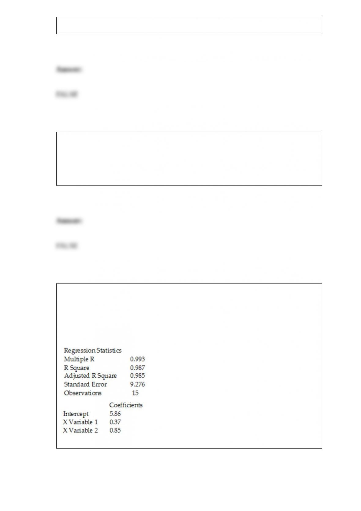
TABLE 16-11
The manager of a health club has recorded mean attendance in newly introduced step
classes over the last 15 months: 32.1, 39.5, 40.3, 46.0, 65.2, 73.1, 83.7, 106.8, 118.0,
133.1, 163.3, 182.8, 205.6, 249.1, and 263.5. She then used Microsoft Excel to obtain
the following partial output for both a first- and second-order autoregressive model.
SUMMARY OUTPUT – 2nd Order Model
SUMMARY OUTPUT – 1st Order Model
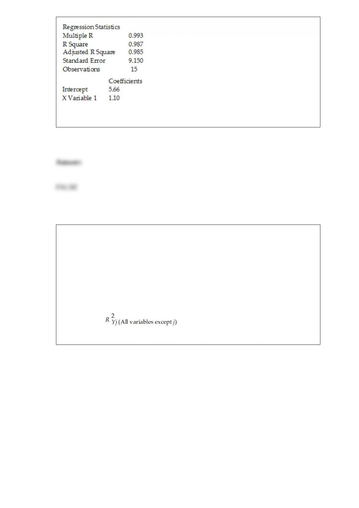
True or False: Referring to Table 16-11, based on the parsimony principle, the
second-order model is the better model for making forecasts.
TABLE 17-10
Given below are results from the regression analysis where the dependent variable is
the number of weeks a worker is unemployed due to a layoff (Unemploy) and the
independent variables are the age of the worker (Age), the number of years of education
received (Edu), the number of years at the previous job (Job Yr), a dummy variable for
marital status (Married: 1 = married, 0 = otherwise), a dummy variable for head of
household (Head: 1 = yes, 0 = no) and a dummy variable for management position
(Manager: 1 = yes, 0 = no). We shall call this Model 1. The coefficient of partial
determination ( ) of each of the 6 predictors are, respectively,
0.2807, 0.0386, 0.0317, 0.0141, 0.0958, and 0.1201.
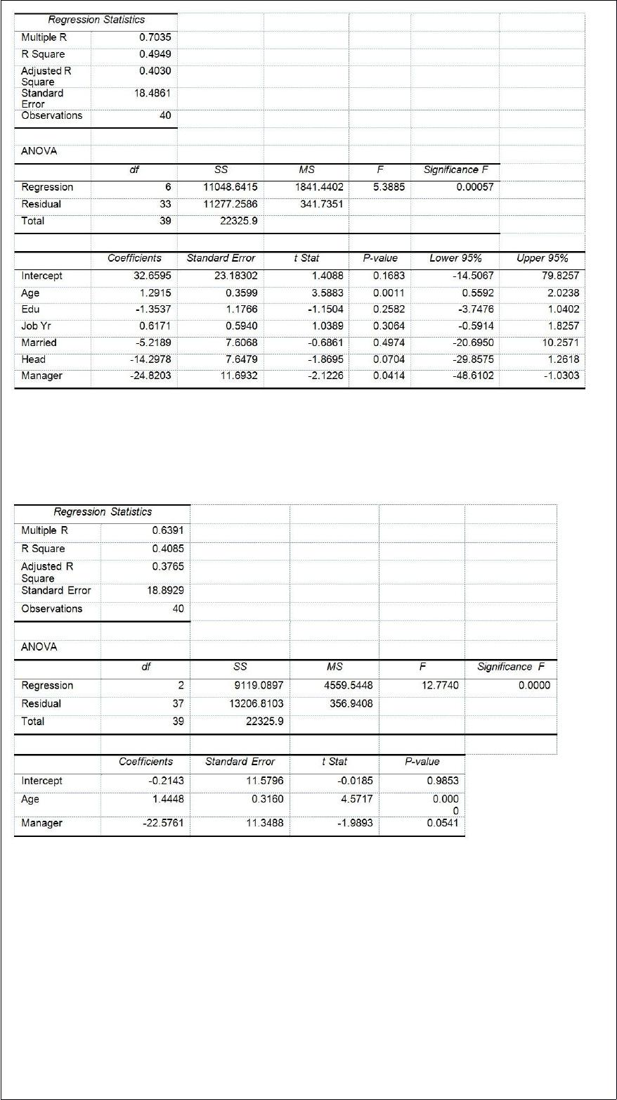
Model 2 is the regression analysis where the dependent variable is Unemploy and the
independent variables are Age and Manager. The results of the regression analysis are
given below:
Referring to Table 17-10, Model 1, which of the following is the correct null hypothesis
to test whether being married or not makes a difference in the mean number of weeks a
worker is unemployed due to a layoff while holding constant the effect of all the other
independent variables?
A) H0 : β1 = 0
B) H0 : β2 = 0
C) H0 : β3 = 0

D) H0 : β4 = 0
Major league baseball salaries averaged $3.26 million with a standard deviation of $1.2
million in a recent year. Suppose a sample of 100 major league players was taken. Find
the approximate probability that the mean salary of the 100 players exceeded $4.0
million.
A) approximately 0
B) 0.0228
C) 0.9772
D) approximately 1
In selecting an appropriate forecasting model, the following approaches are suggested:
A) Perform a residual analysis.
B) Measure the size of the forecasting error.
C) Use the principle of parsimony.
D) All of the above.

In left-skewed distributions, which of the following is the correct statement?
A) The distance from Q1 to Q2 is smaller than the distance from Q2 to Q3.
B) The distance from the smallest observation to Q1 is larger than the distance from Q3
to the largest observation.
C) The distance from the smallest observation to Q2 is less than the distance from Q2 to
the largest observation.
D) The distance from Q1 to Q3 is twice the distance from Q1 to Q2.
TABLE 18-6
The maker of a packaged candy wants to evaluate the quality of her production process.
On each of 16 consecutive days, she samples 600 bags of candy and determines the
number in each day’s sample that she considers to be of poor quality. The data that she
developed follow.

Referring to Table 18-6, a p control chart is to be constructed for these data. The lower
control limit is ________, while the upper control limit is ________.
TABLE 18-4
A factory supervisor is concerned that the time it takes workers to complete an
important production task (measured in seconds) is too erratic and adversely affects
expected profits. The supervisor proceeds by randomly sampling 5 individuals per hour
for a period of 10 hours. The sample mean and range for each hour are listed below.
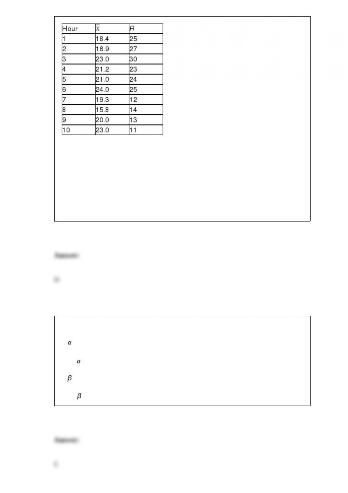
She also decides that lower and upper specification limit for the critical-to-quality
variable should be 10 and 30 seconds, respectively.
Referring to Table 18-4, suppose the supervisor constructs an R chart to see if the
variability in collection times is in-control. What are the lower and upper control limits
for this R chart?
A) -2.33, 43.13
B) -2.28, 42.28
C) 0, 42.28
D) 0, 43.13
The symbol for the probability of committing a Type II error of a statistical test is
A) .
B) 1 – .
C) .
D) 1 – .

Referring to Table 14-18, which of the following is the correct
interpretation for the Toe90 slope coe2cient?
TABLE 14-18
A logistic regression model was estimated in order to predict the
probability that a randomly chosen university or college would be a
private university using information on mean total Scholastic Aptitude
Test score (SAT) at the university or college and whether the TOEFL
criterion is at least 90 (Toe90 = 1 if yes, 0 otherwise). The
dependent variable, Y, is school type (Type = 1 if private and 0
otherwise).
The PHStat output is given below:
A) Holding constant the e”ect of SAT, the estimated mean value of
school type is 0.1928 higher when the school has a TOEFL criterion
that is at least 90.
B) Holding constant the e”ect of SAT, the estimated school type
increases by 0.1928 when the school has a TOEFL criterion that is at
least 90.
C) Holding constant the e”ect of SAT, the estimated natural
logarithm of the odds ratio of the school being a private school is
0.1928 higher for a school that has a TOEFL criterion that is at least
90 than one that does not.
D) Holding constant the e”ect of SAT, the estimated probability of the
school being a private school is 0.1928 higher for a school that has a
TOEFL criterion that is at least 90 than one that does not.

Which of the following sampling methods will more likely be susceptible to ethical
violation when used to form conclusions about the entire population?
A) simple random sample
B) cluster sample
C) systematic sample
D) convenience sample
TABLE 9-2
A student claims that he can correctly identify whether a person is a business major or
an agriculture major by the way the person dresses. Suppose in actuality that if someone
is a business major, he can correctly identify that person as a business major 87% of the
time. When a person is an agriculture major, the student will incorrectly identify that
person as a business major 16% of the time. Presented with one person and asked to
identify the major of this person (who is either a business or an agriculture major), he
considers this to be a hypothesis test with the null hypothesis being that the person is a
business major and the alternative that the person is an agriculture major.
Referring to Table 9-2, what is the “actual confidence coefficient”?
A) 0.13
B) 0.16
C) 0.84
D) 0.87
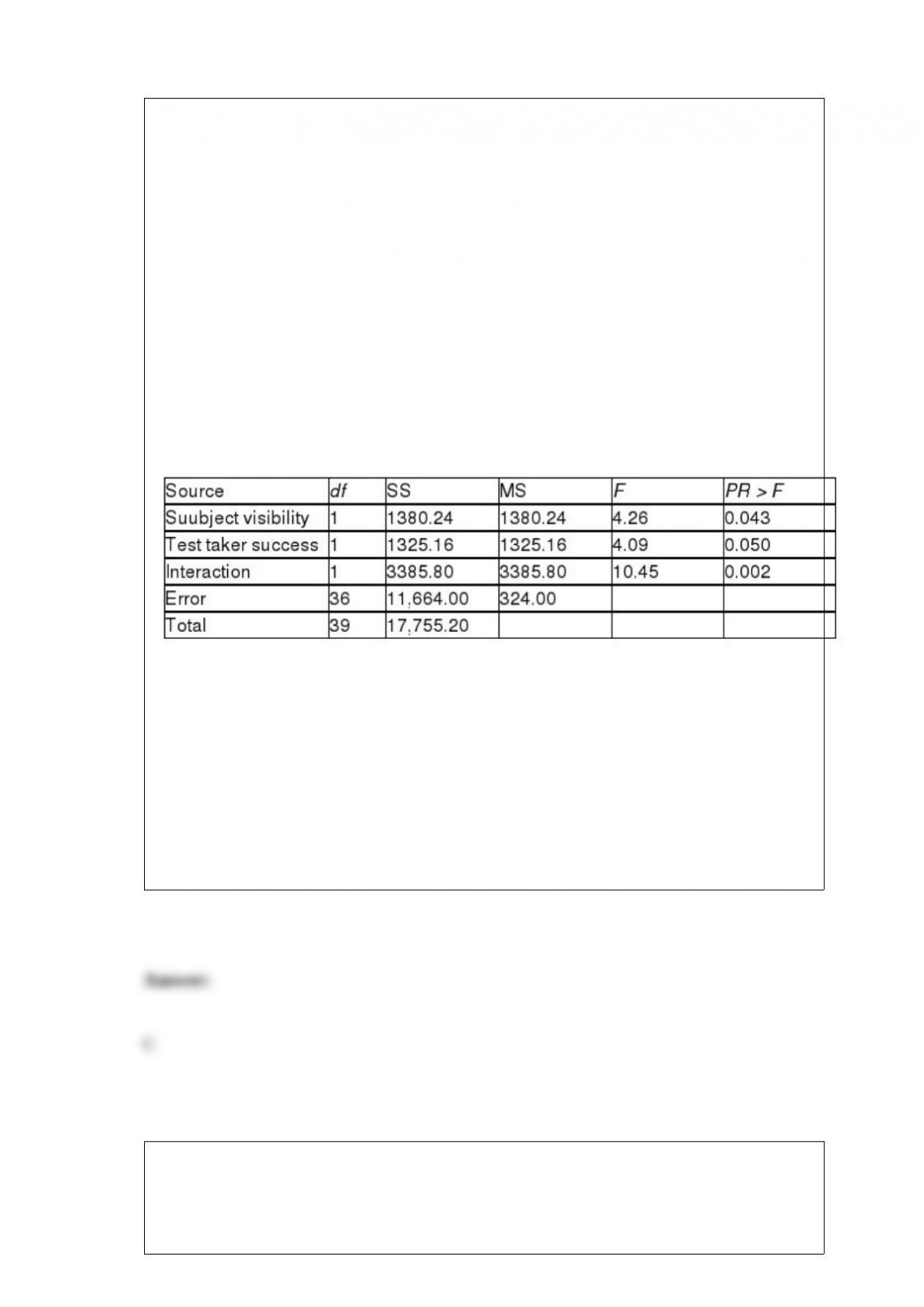
TABLE 11-6
Psychologists have found that people are generally reluctant to transmit bad news to
their peers. This phenomenon has been termed the “MUM effect.” To investigate the
cause of the MUM effect, 40 undergraduates at Duke University participated in an
experiment. Each subject was asked to administer an IQ test to another student and then
provide the test taker with his or her percentile score. Unknown to the subject, the test
taker was a bogus student who was working with the researchers. The experimenters
manipulated two factors: subject visibility and success of test taker, each at two
levels. Subject visibility was either visible or not visible to the test taker. Success of the
test taker was either top 20% or bottom 20%. Ten subjects were randomly assigned to
each of the 2 x 2 = 4 experimental conditions, then the time (in seconds) between the
end of the test and the delivery of the percentile score from the subject to the test taker
was measured. (This variable is called the latency to feedback.) The data were
subjected to appropriate analyses with the following results.
Referring to Table 11-6, what type of experimental design was employed in this study?
A) completely randomized design with 4 treatments
B) randomized block design with four treatments and 10 blocks
C) 2 x 2 factorial design with 10 observations
D) None of the above
TABLE 12-20
A filling machine at a local soft drinks company is calibrated to fill the cans at a mean
amount of 12 fluid ounces and a standard deviation of 0.5 ounces. The company wants

to test whether the standard deviation of the amount filled by the machine is 0.5 ounces.
A random sample of 15 cans filled by the machine reveals a standard deviation of 0.67
ounces.
Referring to Table 12-20, which is the appropriate test to use?
A) X2 test of independence
B) McNemar test
C) Wilcoxon rank sum test
D) X2 test of population variance
A survey claims that 9 out of 10 doctors recommend aspirin for their patients with
headaches. To test this claim, a random sample of 100 doctors results in 83 who
indicate that they recommend aspirin. Which of the following tests will you perform?
A) t test for the mean
B) Z test for the proportion
C) Pooled-variance t test
D) Separate-variance t test
The t test for the difference between the means of 2 independent populations assumes
that the respective
A) sample sizes are equal.
B) sample variances are equal.

C) populations are approximately normal.
D) All of the above.
An entrepreneur is considering the purchase of a coin-operated laundry. The current
owner claims that over the past 5 years, the mean daily revenue was $675 with a
standard deviation of $75. A sample of 30 days reveals a daily mean revenue of $625
and a standard deviation of $70. Which of the following tests will be the most
appropriate?
A) t test for the mean
B) Z test for the proportion
C) Pooled-variance t test
D) Separate-variance t test
TABLE 18-3
A quality control analyst for a light bulb manufacturer is concerned that the time it takes
to produce a batch of light bulbs is too erratic. Accordingly, the analyst randomly
surveys 10 production periods each day for 14 days and records the sample mean and
range for each day.
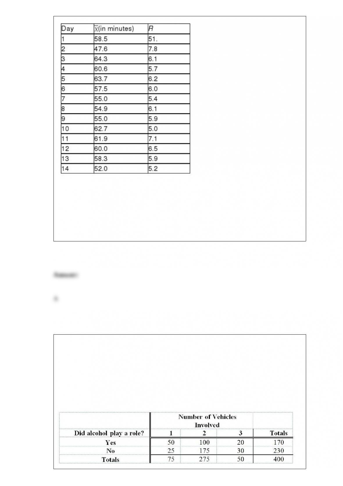
Referring to Table 18-3, suppose the sample mean and range data were based on 11
observations per day instead of 10. How would this change affect the lower and upper
control limits of the R chart?
A) LCL would increase; UCL would decrease.
B) LCL would remain the same; UCL would decrease.
C) Both LCL and UCL would remain the same.
D) LCL would decrease; UCL would increase.
TABLE 4-1
Mothers Against Drunk Driving is a very visible group whose main focus is to educate
the public about the harm caused by drunk drivers. A study was recently done that
emphasized the problem we all face with drinking and driving. Four hundred accidents
that occurred on a Saturday night were analyzed. Two items noted were the number of
vehicles involved and whether alcohol played a role in the accident. The numbers are
shown below:
Referring to Table 4-1, what proportion of accidents involved alcohol or a single
vehicle?
A) 25/400 or 6.25%
B) 50/400 or 12.5%
C) 195/400 or 48.75%
D) 245/400 or 61.25%
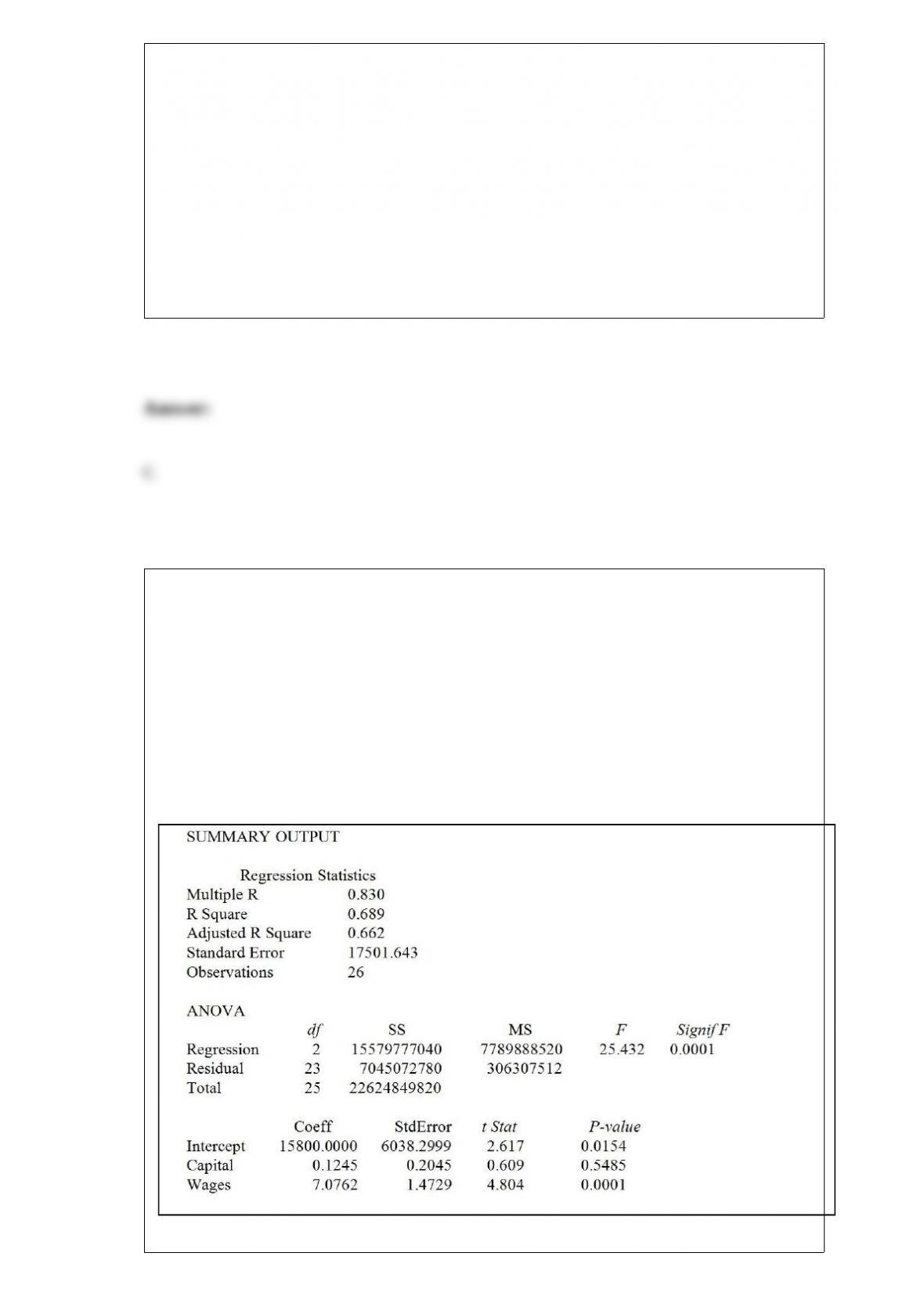
Referring to Table 14-5, when the microeconomist used a simple linear regression
model with sales as the dependent variable and wages as the independent variable, she
obtained an r2 value of 0.601. What additional percentage of the total variation of sales
has been explained by including capital spending in the multiple regression?
TABLE 14-5
A microeconomist wants to determine how corporate sales are influenced by capital and
wage spending by companies. She proceeds to randomly select 26 large corporations
and record information in millions of dollars. The Microsoft Excel output below shows
results of this multiple regression.
A) 60.1%
B) 31.1%
C) 22.9%
D) 8.8%
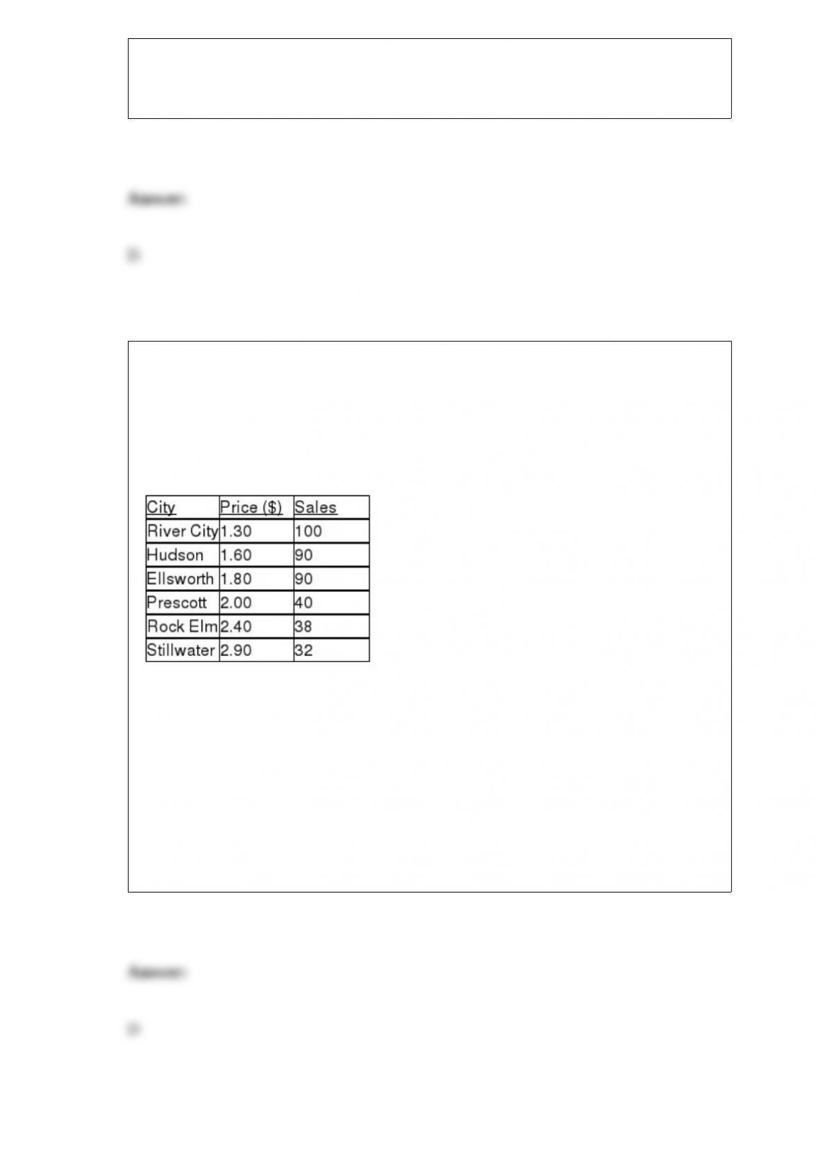
TABLE 13-2
A candy bar manufacturer is interested in trying to estimate how sales are influenced by
the price of their product. To do this, the company randomly chooses 6 small cities and
offers the candy bar at different prices. Using candy bar sales as the dependent variable,
the company will conduct a simple linear regression on the data below:
Referring to Table 13-2, what is the standard error of the estimate, SYX, for the data?
A) 0.784
B) 0.885
C) 12.650
D) 16.299
The amount of time required for an oil and filter change on an automobile is normally
distributed with a mean of 45 minutes and a standard deviation of 10 minutes. A
random sample of 16 cars is selected. 90% of the sample means will be greater than
what value?
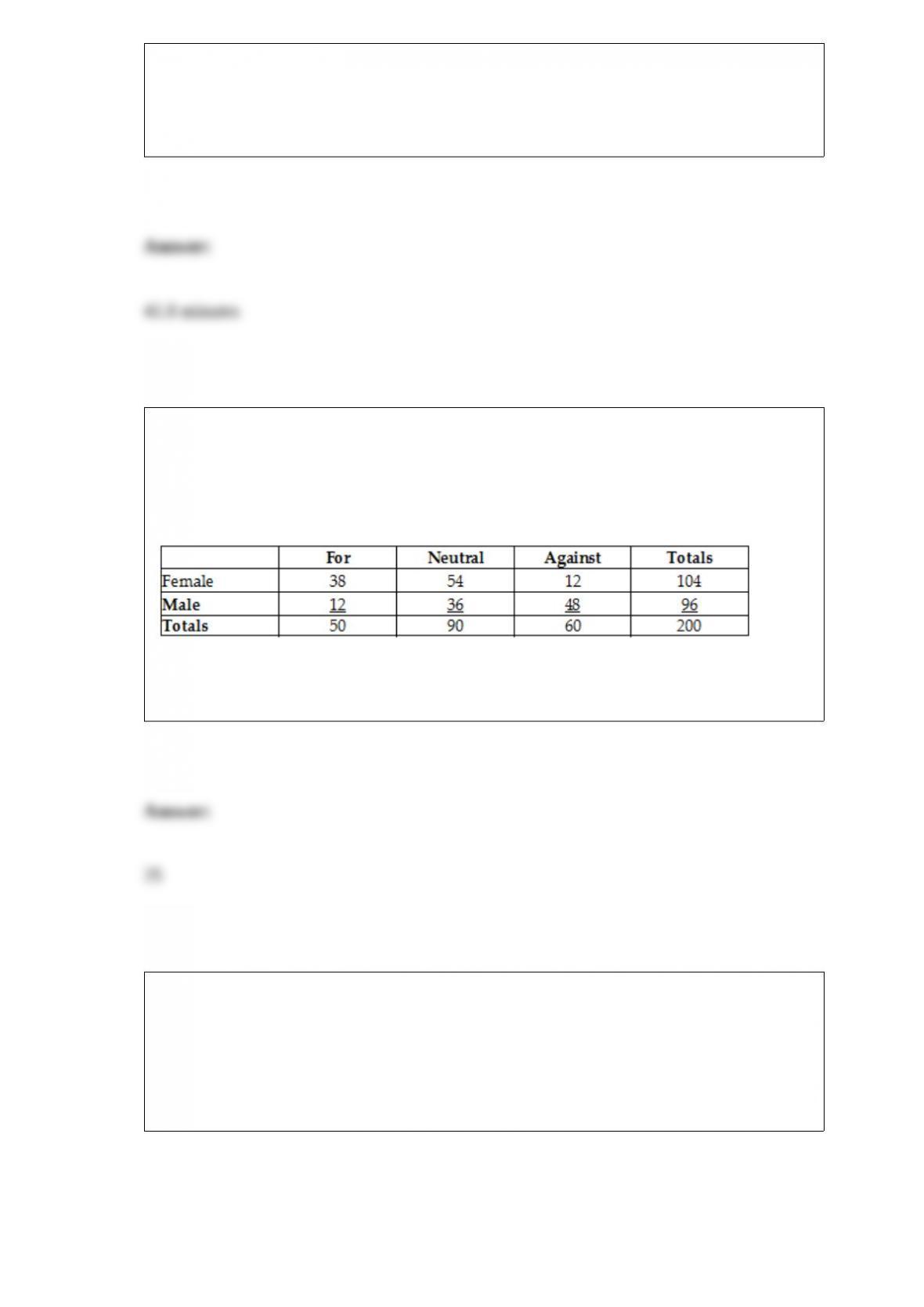
TABLE 2-12
The table below contains the opinions of a sample of 200 people broken down by
gender about the latest congressional plan to eliminate anti-trust exemptions for
professional baseball.
Referring to Table 2-12, if the sample is a good representation of the population, we can
expect ________ percent of the population will be for the plan.
TABLE 11-3
As part of an evaluation program, a sporting goods retailer wanted to compare the
downhill coasting speeds of 4 brands of bicycles. She took 3 of each brand and
determined their maximum downhill speeds. The results are presented in miles per hour
in the table below.
Referring to Table 11-3, the sporting goods retailer decided to perform an ANOVA F
test. The amount of total variation or SST is ________.
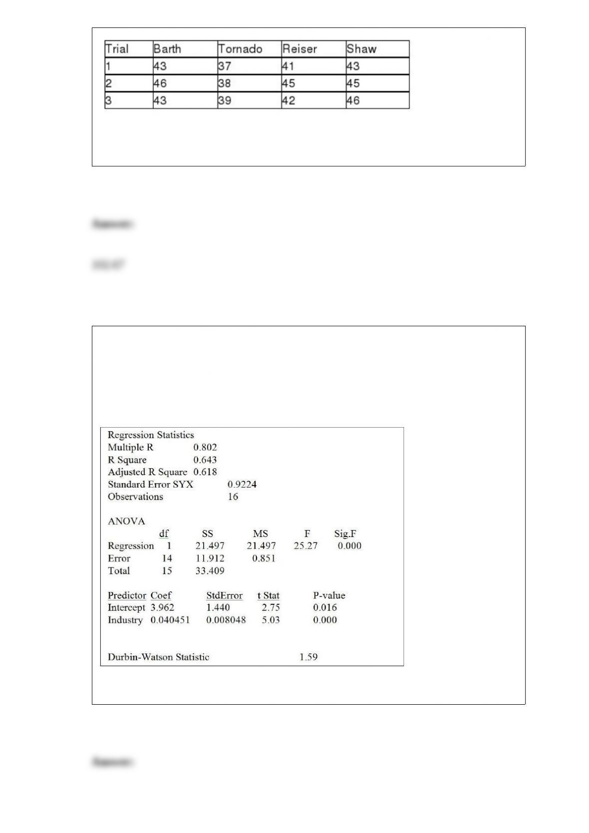
TABLE 13-5
The managing partner of an advertising agency believes that his company’s sales are
related to the industry sales. He uses Microsoft Excel to analyze the last 4 years of
quarterly data (i.e., n = 16) with the following results:
Referring to Table 13-5, the coefficient of determination is ________.
A personal computer user survey was conducted. Hours of personal computer use per
week is an example of a ________ numerical variable.
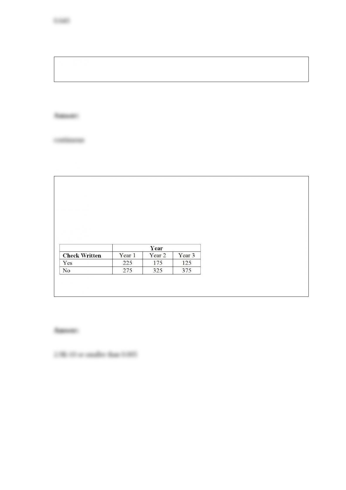
TABLE 12-6
According to an article in Marketing News, fewer checks are being written at the
grocery store checkout than in the past. To determine whether there is a difference in
the proportion of shoppers who pay by check among three consecutive years at a 0.05
level of significance, the results of a survey of 500 shoppers in three consecutive years
are obtained and presented below.
Referring to Table 12-6, what is the p-value of the test statistic?