Unlock document.
This document is partially blurred.
Unlock all pages and 1 million more documents.
Get Access

TABLE 14-19
The marketing manager for a nationally franchised lawn service
company would like to study the characteristics that di erentiate
home owners who do and do not have a lawn service. A random
sample of 30 home owners located in a suburban area near a large
city was selected; 11 did not have a lawn service (code 0) and 19 had
a lawn service (code 1). Additional information available concerning
these 30 home owners includes family income (Income, in thousands
of dollars) and lawn size (Lawn Size, in thousands of square feet).
The PHStat output is given below:
True or False: Referring to Table 14-19, there is not enough evidence
to conclude that the model is not a good-1tting model at a 0.05 level
of signiticance.
True or False: The larger the number of observations in a numerical data set, the larger
the number of class intervals needed for a grouped frequency distribution.
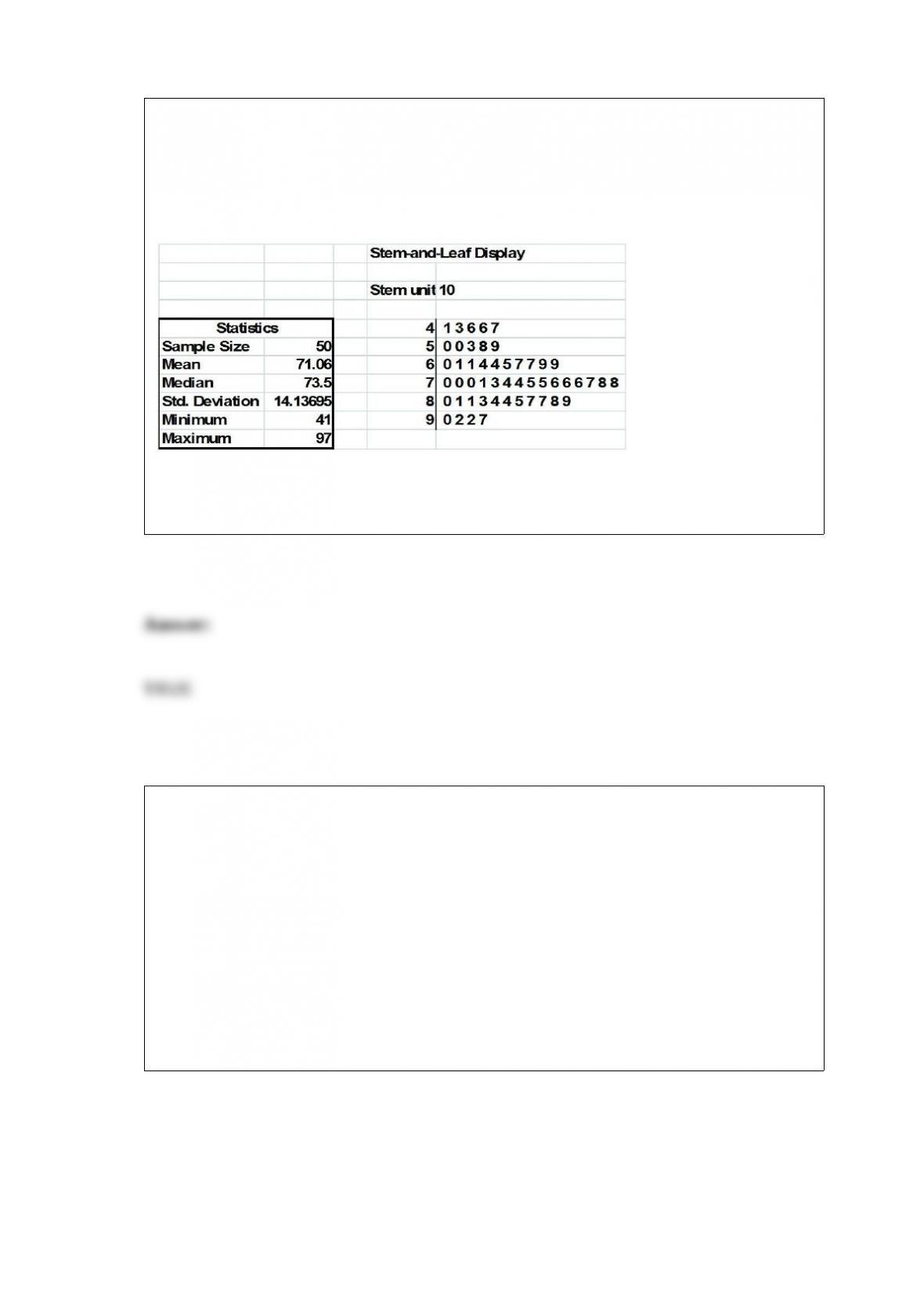
TABLE 2-18
The stem-and-leaf display below shows the result of a survey of 50 students on their
satisfaction with their school, with the higher scores representing a higher level of
satisfaction.
True or False: Referring to Table 2-18, the level of satisfaction is concentrated around
75.
TABLE 14-15
The superintendent of a school district wanted to predict the
percentage of students passing a sixth-grade proficiency test. She
obtained the data on percentage of students passing the proficiency
test (% Passing), mean teacher salary in thousands of dollars
(Salaries), and instructional spending per pupil in thousands of dollars
(Spending) of 47 schools in the state.
Following is the multiple regression output with Y = % Passing as the
dependent variable, X1 = Salaries and X2 = Spending:

True or False: Referring to Table 14-15, there is suffcient evidence
that the percentage of students passing the proficiency test depends
on both of the explanatory variables at a 5% level of signiticance.
True or False: To determine the probability of getting between 3 and 4 events of interest
in a binomial distribution, you will find the area under the normal curve between X =
3.5 and 4.5.
True or False: The mean of the sampling distribution of a sample proportion is the
population proportion, .
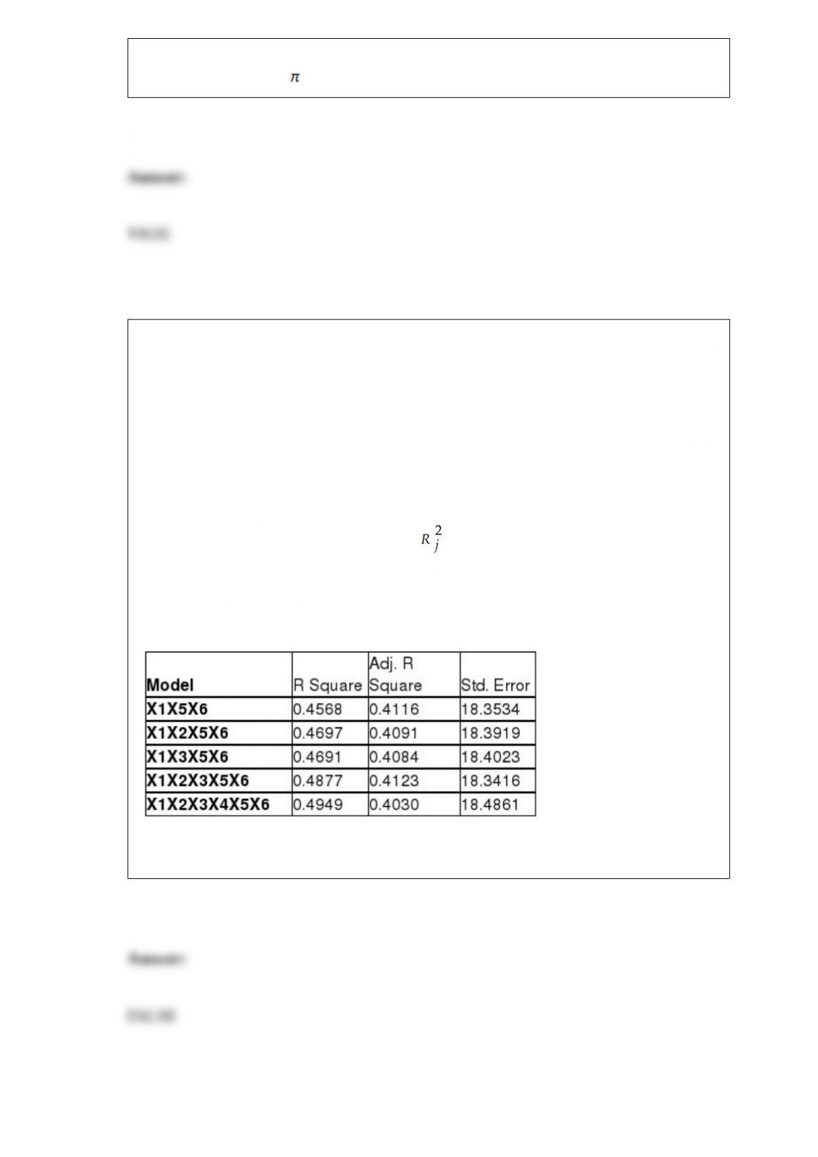
TABLE 15-6
Given below are results from the regression analysis on 40 observations where the
dependent variable is the number of weeks a worker is unemployed due to a layoff (Y)
and the independent variables are the age of the worker (X1), the number of years of
education received (X2), the number of years at the previous job (X3), a dummy variable
for marital status (X4: 1 = married, 0 = otherwise), a dummy variable for head of
household (X5: 1 = yes, 0 = no) and a dummy variable for management position (X6: 1
= yes, 0 = no).
The coefficient of multiple determination ( ) for the regression model using each of
the 6 variables Xj as the dependent variable and all other X variables as independent
variables are, respectively, 0.2628, 0.1240, 0.2404, 0.3510, 0.3342 and 0.0993.
The partial results from best-subset regression are given below:
True or False: Referring to Table 15-6, the model that includes all six independent
variablesshould be selected using the adjusted r2 statistic.

TABLE 8-4
The actual voltages of power packs labeled as 12 volts are as follows: 11.77, 11.90,
11.64, 11.84, 12.13, 11.99, and 11.77.
True or False: Referring to Table 8-4, a 90% confidence interval calculated from the
same data would be narrower than a 99% confidence interval.
True or False: The Guidelines for Developing Visualizations recommend always
including a scale for each axis if the chart contains axes.
TABLE 8-9
A university wanted to find out the percentage of students who felt comfortable
reporting cheating by their fellow students. A survey of 2,800 students was conducted
and the students were asked if they felt comfortable reporting cheating by their fellow
students. The results were 1,344 answered "Yes" and 1,456 answered "No."
True or False: Referring to Table 8-9, the parameter of interest is the proportion of the
student population who feel comfortable reporting cheating by their fellow students.
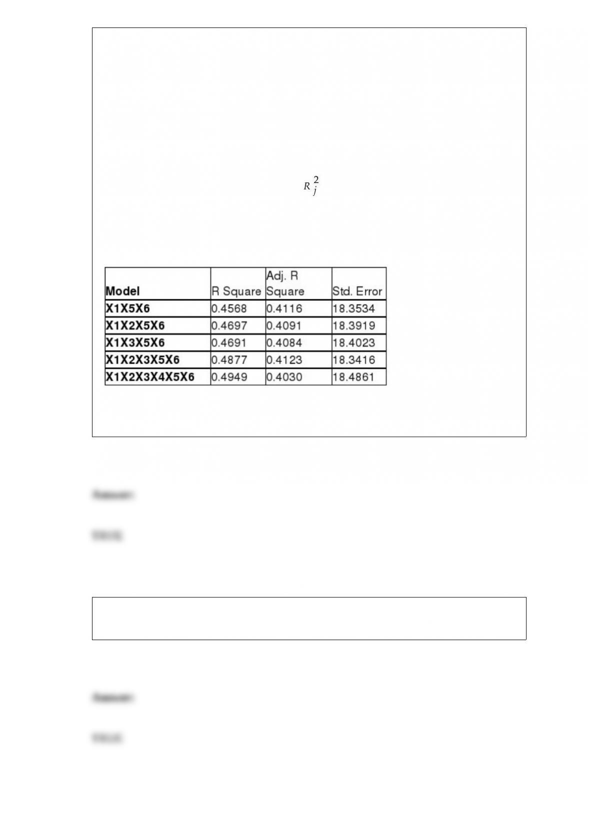
TABLE 15-6
Given below are results from the regression analysis on 40 observations where the
dependent variable is the number of weeks a worker is unemployed due to a layoff (Y)
and the independent variables are the age of the worker (X1), the number of years of
education received (X2), the number of years at the previous job (X3), a dummy variable
for marital status (X4: 1 = married, 0 = otherwise), a dummy variable for head of
household (X5: 1 = yes, 0 = no) and a dummy variable for management position (X6: 1
= yes, 0 = no).
The coefficient of multiple determination ( ) for the regression model using each of
the 6 variables Xj as the dependent variable and all other X variables as independent
variables are, respectively, 0.2628, 0.1240, 0.2404, 0.3510, 0.3342 and 0.0993.
The partial results from best-subset regression are given below:
True or False: Referring to Table 15-6, the model that includes X1, X5 and X6 should be
among the appropriate models using the Mallow's Cp statistic.
True or False: The median of a data set with 20 items would be the average of the 10th
and the 11th items in the ordered array.
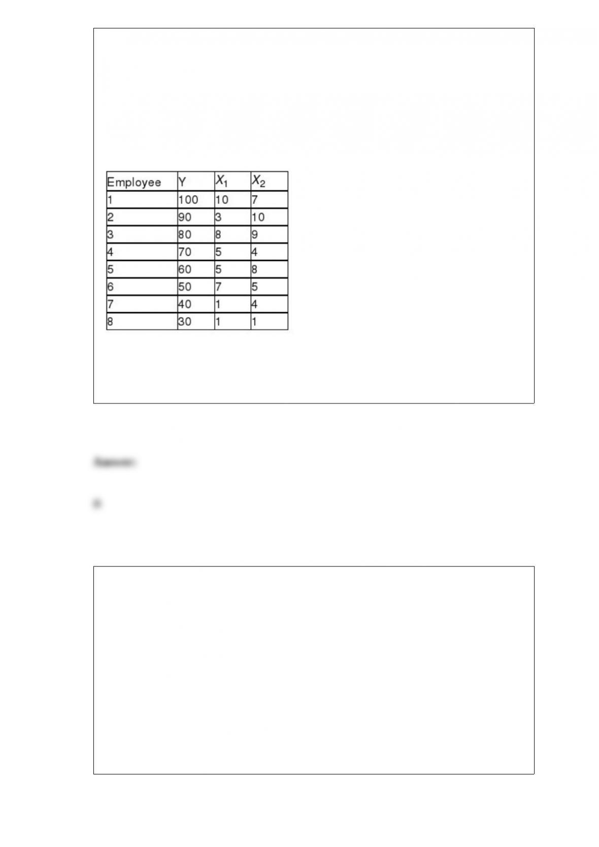
Referring to Table 14-1, for these data, what is the estimated coefficient for the variable
representing years an employee has been with the company, b1?
TABLE 14-1
A manager of a product sales group believes the number of sales made by an employee
(Y) depends on how many years that employee has been with the company (X1) and
how he/she scored on a business aptitude test (X2). A random sample of 8 employees
provides the following:
A) 0.998
B) 3.103
C) 4.698
D) 21.293
A financial analyst is presented with information on the past records of 60 start-up
companies and told that in fact only 3 of them have managed to become highly
successful. He selected 3 companies from this group as the candidates for success. To
analyze his ability to spot the companies that will eventually become highly successful,
he will use what type of probability distribution?
A) Binomial distribution
B) Poisson distribution
C) Hypergeometric distribution
D) None of the above
TABLE 16-12
A local store developed a multiplicative time-series model to forecast its revenues in
future quarters, using quarterly data on its revenues during the 5-year period from 2008
to 2012. The following is the resulting regression equation:
log10 = 6.102 + 0.012 X - 0.129 1 - 0.054 2 + 0.098 3
where is the estimated number of contracts in a quarter
X is the coded quarterly value with X = 0 in the first quarter of 2008
1 is a dummy variable equal to 1 in the first quarter of a year and 0 otherwise
2 is a dummy variable equal to 1 in the second quarter of a year and 0 otherwise
is a dummy variable equal to 1 in the third quarter of a year and 0 otherwise
Referring to Table 16-12, the best interpretation of the constant 6.102 in the regression
equation is
A) the fitted value for the first quarter of 2008, prior to seasonal adjustment, is
log10(6.102).
B) the fitted value for the first quarter of 2008, after to seasonal adjustment, is
log10(6.102).
C) the fitted value for the first quarter of 2008, prior to seasonal adjustment, is 106.102.
D) the fitted value for the first quarter of 2008, after to seasonal adjustment, is 106.102.
If the correlation coefficient (r) = 1.00, then
A) all the data points must fall exactly on a straight line with a slope that equals 1.00.
B) all the data points must fall exactly on a straight line with a negative slope.
C) all the data points must fall exactly on a straight line with a positive slope.
D) all the data points must fall exactly on a horizontal straight line with a zero slope.
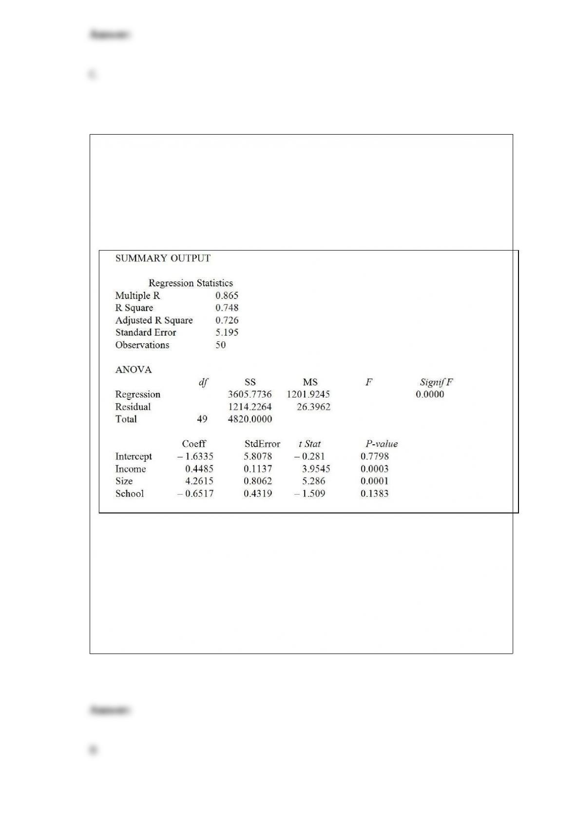
TABLE 17-1
A real estate builder wishes to determine how house size (House) is influenced by
family income (Income), family size (Size), and education of the head of household
(School). House size is measured in hundreds of square feet, income is measured in
thousands of dollars, and education is in years. The builder randomly selected 50
families and ran the multiple regression. Microsoft Excel output is provided below:
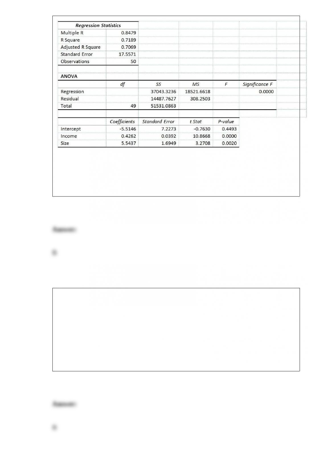
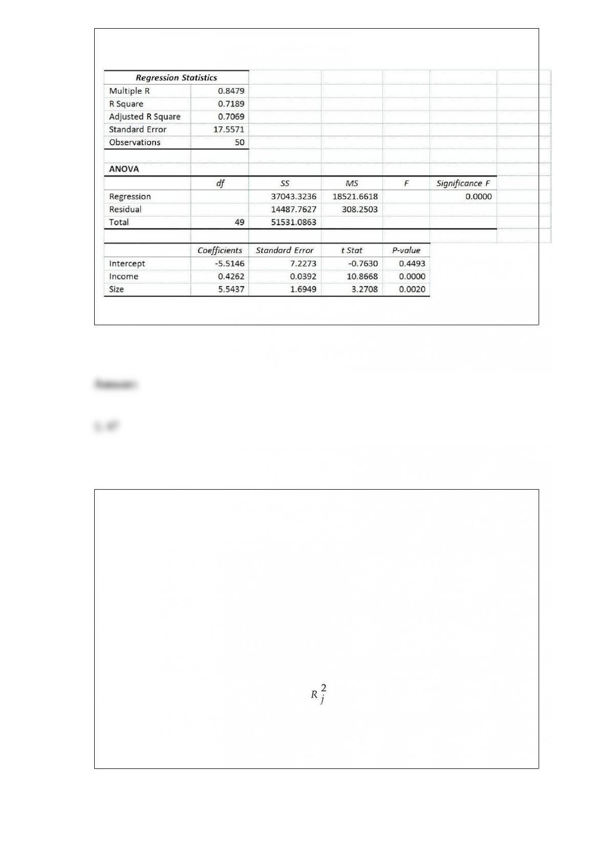
Referring to Table 17-1, when the builder used a simple linear regression model with
house size (House) as the dependent variable and education (School) as the independent
variable, he obtained an r2 value of 23.0%. What additional percentage of the total
variation in house size has been explained by including family size and income in the
multiple regression?
A) 2.8%
B) 51.8%
C) 72.6%
D) 74.8%

A summary measure that is computed to describe a characteristic from only a sample of
the population is called
A) an ordered array.
B) a summary table.
C) a statistic.
D) a parameter.
You have collected data on the number of U.S. households actively using online
banking and/or online bill payment over a 10-year period. Which of the following is the
best for presenting the data?
A) a pie chart
B) a stem-and-leaf display
C) a side-by-side bar chart
D) a time-series plot
If a categorical independent variable contains 2 categories, then ________ dummy
variable(s) will be needed to uniquely represent these categories.
A) 1
B) 2
C) 3
D) 4
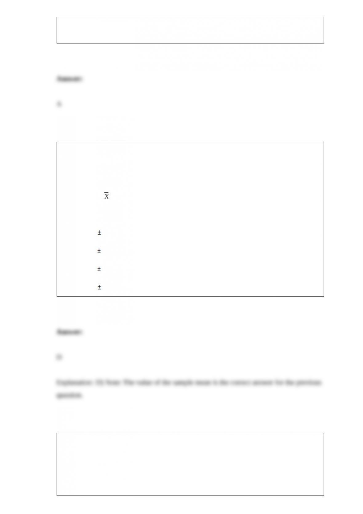
Private colleges and universities rely on money contributed by individuals and
corporations for their operating expenses. Much of this money is put into a fund called
an endowment, and the college spends only the interest earned by the fund. A recent
survey of 8 private colleges in the United States revealed the following endowments (in
millions of dollars): 60.2, 47.0, 235.1, 490.0, 122.6, 177.5, 95.4, and 220.0. Summary
statistics yield = 180.975 and S = 143.042. Calculate a 95% confidence interval for
the mean endowment of all the private colleges in the United States assuming a normal
distribution for the endowments.
A) $180.975 $94.066
B) $180.975 $99.123
C) $180.975 $116.621
D) $180.975 $119.586
TABLE 17-8
The superintendent of a school district wanted to predict the percentage of students
passing a sixth-grade proficiency test. She obtained the data on percentage of students
passing the proficiency test (% Passing), daily mean of the percentage of students
attending class (% Attendance), mean teacher salary in dollars (Salaries), and
instructional spending per pupil in dollars (Spending) of 47 schools in the state.
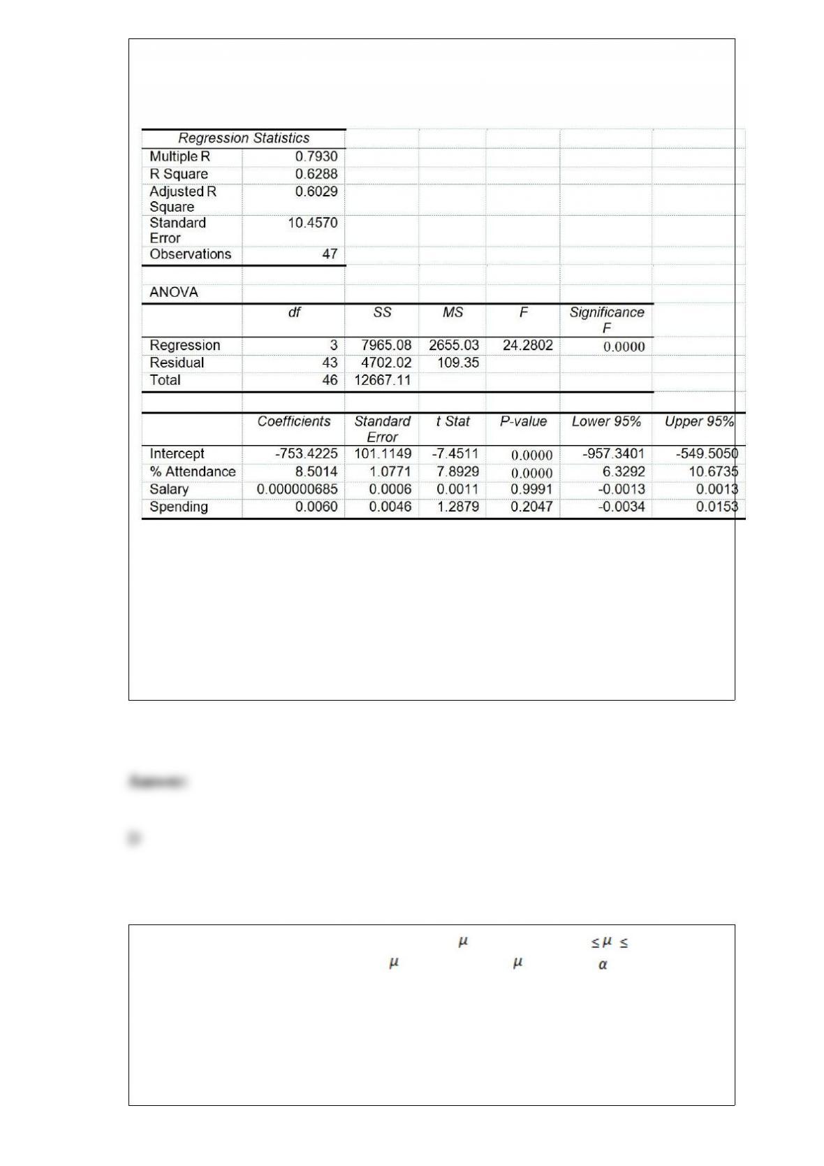
Following is the multiple regression output with Y = % Passing as the dependent
variable, X1 = % Attendance, X2 = Salaries and X3 = Spending:
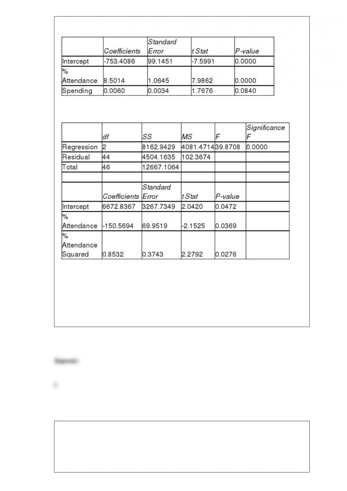
Referring to Table 17-8, which of the following is the correct alternative hypothesis to
determine whether there is a significant relationship between the percentage of students
passing the proficiency test and the entire set of explanatory variables?
A) H1 : β0 = β1 = β2 = β3 ≠0
B) H1 : β1 = β2 = β3 ≠0
C) H1 : At least one of βj ≠0 for j = 0, 1, 2, 3
D) H1 : At least one of βj ≠0 for j = 1, 2, 3
You have created a 95% confidence interval for with the result 10 15. What
decision will you make if we test H0: = 16 versus H1: ≠16 at = 0.10?
A) Reject H0 in favor of H1.
B) Do not reject H0 in favor of H1.
C) Fail to reject H0 in favor of H1.
D) We cannot tell what our decision will be from the information given.
Which of the following is not sensitive to extreme values?
A) the range
B) the standard deviation
C) the interquartile range
D) the coefficient of variation
Referring to Table 14-4, suppose the builder wants to test whether the coefficient on
Size is significantly different from 0. What is the value of the relevant t-statistic?
TABLE 14-4
A real estate builder wishes to determine how house size (House) is influenced by
family income (Income) and family size (Size). House size is measured in hundreds of
square feet and income is measured in thousands of dollars. The builder randomly
selected 50 families and ran the multiple regression. Partial Microsoft Excel output is
provided below:
Also SSR (X1∣ X2) = 36400.6326 and SSR (X2∣ X1) = 3297.7917
A) -0.7630
B) 3.2708
C) 10.8668
D) 60.0864
The standard error of the population proportion will become larger
A) as population proportion approaches 0.
B) as population proportion approaches 0.50.
C) as population proportion approaches 1.00.
D) as the sample size increases.
TABLE 15-4
The superintendent of a school district wanted to predict the percentage of students
passing a sixth-grade proficiency test. She obtained the data on percentage of students
passing the proficiency test (% Passing), daily mean of the percentage of students
attending class (% Attendance), mean teacher salary in dollars (Salaries), and
instructional spending per pupil in dollars (Spending) of 47 schools in the state.
Let Y = % Passing as the dependent variable, X1 = % Attendance, X2 = Salaries and X3
= Spending.
The coefficient of multiple determination ( ) of each of the 3 predictors with all the
other remaining predictors are, respectively, 0.0338, 0.4669, and 0.4743.
The output from the best-subset regressions is given below:
Following is the residual plot for % Attendance:
Following is the output of several multiple regression models:
Model (I):
Model (II):
Model (III):
Referring to Table 15-4, which of the following models should be taken into
consideration using the Mallows' Cp statistic?
A) X1, X3
B) X1, X2, X3
C) Both of the above
D) None of the above
A quality control manager at a plant that produces o-rings is concerned about whether
the diameter of the o-rings that are produced is conformable to the specification. She
has calculated that the average diameter of the o-rings is 4.2 centimeters. She also
knows that approximately 95% of the o-rings have diameters that fall between 3.2 and
5.2 centimeters and almost all of the o-rings have diameters between 2.7 and 5.7

centimeters. When modeling the diameters of the o-rings, which distribution should the
scientists use?
A) Uniform distribution
B) Binomial distribution
C) Normal distribution
D) Exponential distribution
TABLE 10-3
A real estate company is interested in testing whether the mean time that families in
Gotham have been living in their current homes is less than families in Metropolis.
Assume that the two population variances are equal. A random sample of 100 families
from Gotham and a random sample of 150 families in Metropolis yield the following
data on length of residence in current homes.
Gotham: G = 35 months, = 900 Metropolis: M = 50 months, = 1050
Referring to Table 10-3, what is a point estimate for the mean of the sampling
distribution of the difference between the 2 sample means?
A) -22
B) -10
C) -15
D) 0
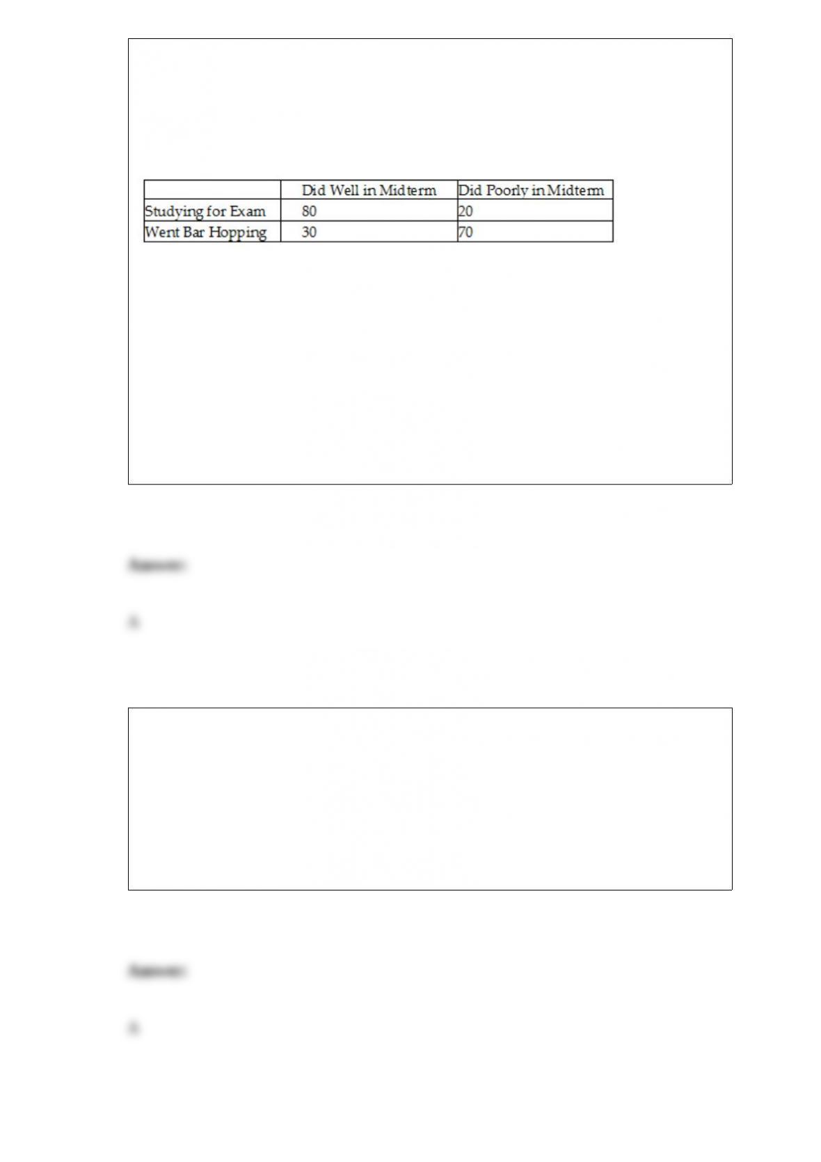
TABLE 2-6
A sample of 200 students at a Big-Ten university was taken after the midterm to ask
them whether they went bar hopping the weekend before the midterm or spent the
weekend studying, and whether they did well or poorly on the midterm. The following
table contains the result.
Referring to Table 2-6, ________ percent of the students in the sample went bar
hopping the weekend before the midterm and did well on the midterm.
A) 15
B) 27.27
C) 30
D) 50
Data on the amount of money made in a year by 1,000 families in a small town were
collected. You want to know how much each family will get if the money made by all
the 1,000 families is pooled together and then evenly redistributed back to them. Which
of the following would you compute?
A) Arithmetic mean
B) Median
C) Interquartile range
D) Coefficient of correlation
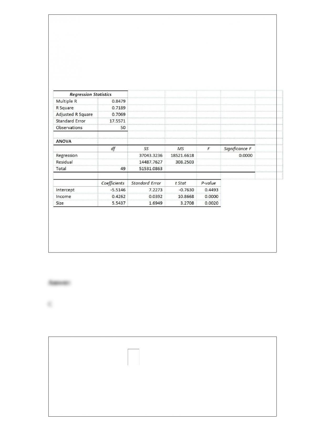
Referring to Table 14-4, suppose the builder wants to test whether the coefficient on
Income is significantly different from 0. What is the value of the relevant t-statistic?
TABLE 14-4
A real estate builder wishes to determine how house size (House) is influenced by
family income (Income) and family size (Size). House size is measured in hundreds of
square feet and income is measured in thousands of dollars. The builder randomly
selected 50 families and ran the multiple regression. Partial Microsoft Excel output is
provided below:
Also SSR (X1∣ X2) = 36400.6326 and SSR (X2∣ X1) = 3297.7917
A) -0.7630
B) 3.2708
C) 10.8668
D) 60.0864
Referring to Table 14-7, the value of the adjusted coefficient of
multiple determination, , is ________.
TABLE 14-7
The department head of the accounting department wanted to see if
she could predict the GPA of students using the number of course
units (credits) and total SAT scores of each. She takes a sample of

students and generates the following Microsoft Excel output:
TABLE 13-4
The managers of a brokerage firm are interested in finding out if the number of new
clients a broker brings into the firm affects the sales generated by the broker. They
sample 12 brokers and determine the number of new clients they have enrolled in the
last year and their sales amounts in thousands of dollars. These data are presented in the
table that follows.
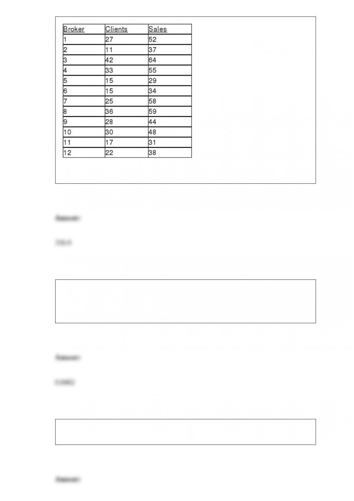
Referring to Table 13-4, the error or residual sum of squares (SSE) is ________.
A debate team of 4 members for a high school will be chosen randomly from a potential
group of 15 students. Ten of the 15 students have no prior competition experience while
the others have some degree of experience. What is the probability that at least 1 of the
members chosen for the team have some prior competition experience?
If the residuals in a regression analysis of time-ordered data are not correlated, the value
of the Durbin-Watson D statistic should be near ________.
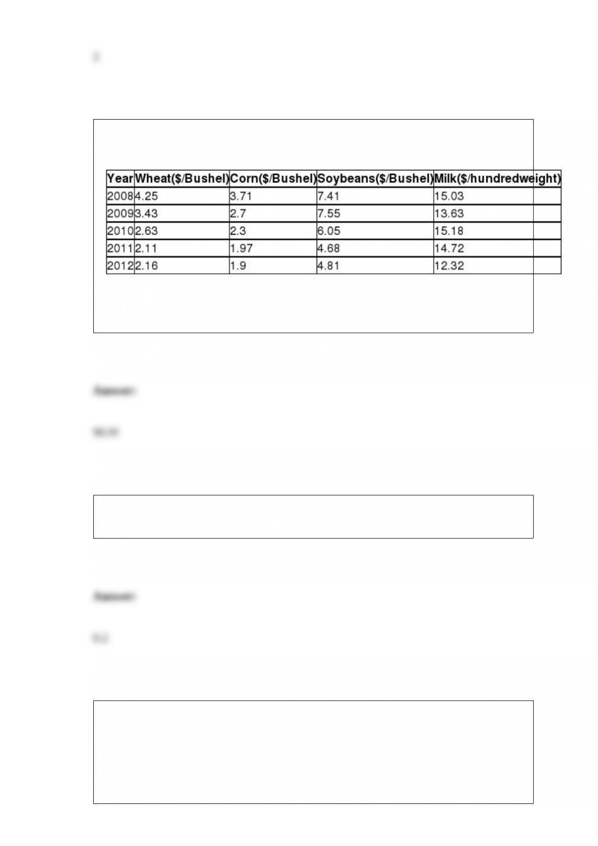
TABLE 16-16
Given below are the prices of a basket of four food items from 2008 to 2012.
Referring to Table 16-16, what is the Laspeyres price index for the basket of four food
items in 2010 that consisted of 50 bushels of wheat, 30 bushels of corn, 40 bushels of
soybeans and 80 hundredweight of milk in 2008 using 2008 as the base year?
Suppose A and B are independent events where P(A) = 0.4 and P(B) = 0.5. Then P(A
and B) = ________.
TABLE 17-9
What are the factors that determine the acceleration time (in sec.) from 0 to 60 miles per
hour of a car? Data on the following variables for 171 different vehicle models were
collected:
Accel Time: Acceleration time in sec.
Cargo Vol: Cargo volume in cu. ft.
HP: Horsepower
MPG: Miles per gallon
SUV: 1 if the vehicle model is an SUV with Coupe as the base when SUV and Sedan
are both 0
Sedan: 1 if the vehicle model is a sedan with Coupe as the base when SUV and Sedan
are both 0
The regression results using acceleration time as the dependent variable and the
remaining variables as the independent variables are presented below.
The various residual plots are as shown below.
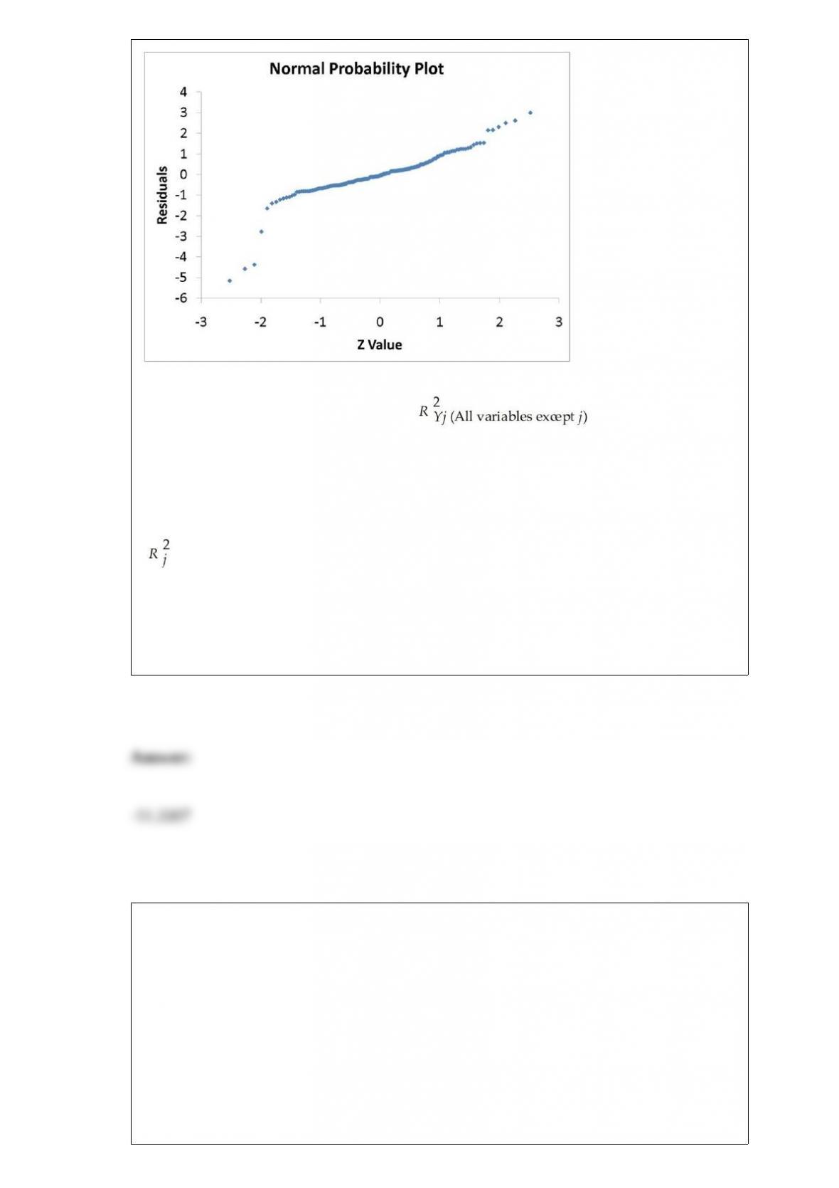
The coefficient of partial determination ( ) of each of the 5
predictors are, respectively, 0.0380, 0.4376, 0.0248, 0.0188, and 0.0312.
The coefficient of multiple determination for the regression model using each of the 5
variables Xj as the dependent variable and all other X variables as independent variables
( ) are, respectively, 0.7461, 0.5676, 0.6764, 0.8582, 0.6632.
Referring to Table 17-9, what is the value of the test statistic to determine whether HP
makes a significant contribution to the regression model in the presence of the other
independent variables at a 5% level of significance?
Referring to Table 14-4, the partial F test for
H0 : Variable X1 does not significantly improve the model after variable X2 has been
included
H1 : Variable X1 significantly improves the model after variable X2 has been included
has ________ and ________ degrees of freedom.
TABLE 14-4
A real estate builder wishes to determine how house size (House) is influenced by
family income (Income) and family size (Size). House size is measured in hundreds of
square feet and income is measured in thousands of dollars. The builder randomly
selected 50 families and ran the multiple regression. Partial Microsoft Excel output is
provided below:
Also SSR (X1∣ X2) = 36400.6326 and SSR (X2∣ X1) = 3297.7917
TABLE 15-5
What are the factors that determine the acceleration time (in sec.) from 0 to 60 miles per
hour of a car? Data on the following variables for 171 different vehicle models were
collected:
Accel Time: Acceleration time in sec.
Cargo Vol: Cargo volume in cu. ft.
HP: Horsepower
MPG: Miles per gallon
SUV: 1 if the vehicle model is an SUV with Coupe as the base when SUV and Sedan
are both 0
Sedan: 1 if the vehicle model is a sedan with Coupe as the base when SUV and Sedan
are both 0
The coefficient of multiple determination ( ) for the regression model using each of
the 5 variables Xj as the dependent variable and all other X variables as independent
variables are, respectively, 0.7461, 0.5676, 0.6764, 0.8582, 0.6632.
Referring to Table 15-5, what is the value of the variance inflationary factor of HP?


