
True or False: A sampling distribution is defined as the probability distribution of
possible sample sizes that can be observed from a given population.
True or False: For a t distribution with 12 degrees of freedom, the area between -2.6810
and 2.1788 is 0.980.
True or False: Ogives are plotted at the midpoints of the class groupings.
TABLE 14-15
The superintendent of a school district wanted to predict the
percentage of students passing a sixth-grade proficiency test. She
obtained the data on percentage of students passing the proficiency
test (% Passing), mean teacher salary in thousands of dollars
(Salaries), and instructional spending per pupil in thousands of dollars
(Spending) of 47 schools in the state.
Following is the multiple regression output with Y = % Passing as the
dependent variable, X1 = Salaries and X2 = Spending:

True or False: Referring to Table 14-15, the alternative hypothesis H1 :
At least one of βj ≠0 for j = 1, 2 implies that percentage of
students passing the proficiency test is related to both of the
explanatory variables.
TABLE 8-6
After an extensive advertising campaign, the manager of a company wants to estimate
the proportion of potential customers that recognize a new product. She samples 120
potential consumers and finds that 54 recognize this product. She uses this sample
information to obtain a 95% confidence interval that goes from 0.36 to 0.54.
True or False: Referring to Table 8-6, the parameter of interest is 54/120 = 0.45.
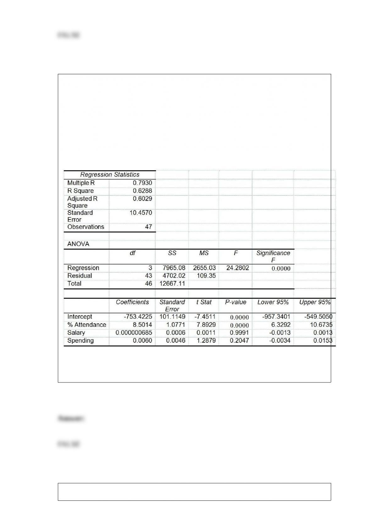
True or False: TABLE 17-8
The superintendent of a school district wanted to predict the percentage of students
passing a sixth-grade proficiency test. She obtained the data on percentage of students
passing the proficiency test (% Passing), daily mean of the percentage of students
attending class (% Attendance), mean teacher salary in dollars (Salaries), and
instructional spending per pupil in dollars (Spending) of 47 schools in the state.
Following is the multiple regression output with Y = % Passing as the dependent
variable, X1 = % Attendance, X2 = Salaries and X3 = Spending:
Referring to Table 17-8, the null hypothesis H0 : β1 = β2 = β3 = 0 implies that the
percentage of students passing the proficiency test is not related to one of the
explanatory variables.
True or False: A multiple regression is called “multiple” because it has several data

points.
TABLE 14-15
The superintendent of a school district wanted to predict the
percentage of students passing a sixth-grade proficiency test. She
obtained the data on percentage of students passing the proficiency
test (% Passing), mean teacher salary in thousands of dollars
(Salaries), and instructional spending per pupil in thousands of dollars
(Spending) of 47 schools in the state.
Following is the multiple regression output with Y = % Passing as the
dependent variable, X1 = Salaries and X2 = Spending:
True or False: Referring to Table 14-15, the null hypothesis should be
rejected at a 5% level of significance when testing whether there is a
significant relationship between percentage of students passing the
proficiency test and the entire set of explanatory variables.

True or False: An insurance company evaluates many variables about a person before
deciding on an appropriate rate for automobile insurance. A representative from a local
insurance agency selected a random sample of 100 insured drivers and recorded, X, the
amount of claims each made in the last 3 years. A Pareto chart can be used to present
this information.
True or False: TABLE 18-7
A supplier of silicone sheets for producers of computer chips wants to evaluate her
manufacturing process. She takes sample sizes of 5 from each day’s output and counts
the number of blemishes on each silicone sheet. The results from 20 days of such
evaluations are presented below.
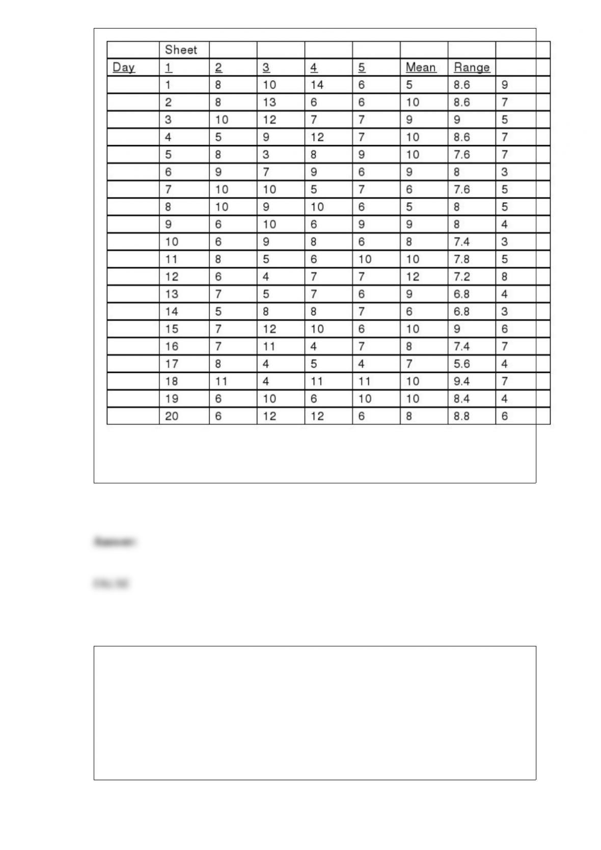
She also decides that the upper specification limit is 10 blemishes.
Referring to Table 18-7, based on the R chart, it appears that the process is out of
control.
TABLE 11-9
The marketing manager of a company producing a new cereal aimed for children wants
to examine the effect of the color and shape of the box’s logo on the approval rating of
the cereal. He combined 4 colors and 3 shapes to produce a total of 12 designs. Each
logo was presented to 2 different groups (a total of 24 groups) and the approval rating
for each was recorded and is shown below. The manager analyzed these data using the
α = 0.05 level of significance for all inferences.
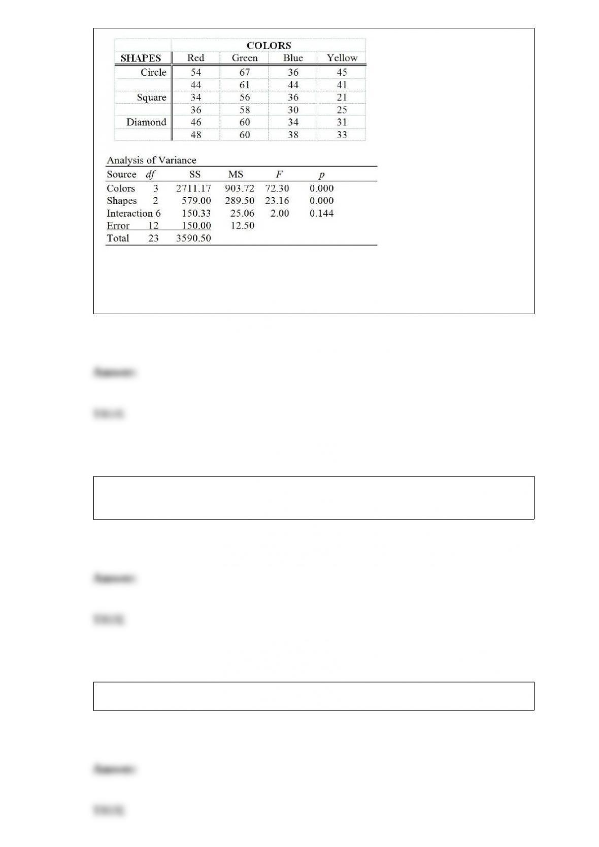
True or False: Referring to Table 11-9, based on the results of the hypothesis test, it
appears that there is a significant effect on the approval rating associated with the color
of the logo.
True or False: The line drawn within the box of the boxplot always represents the
median.
True or False: The coefficient of determination represents the ratio of SSR to SST.

True or False: If remains constant in a binomial distribution, an increase in n will
increase the variance.
In general, which of the following descriptive summary measures cannot be easily
approximated from a boxplot?
A) the variance
B) the range
C) the interquartile range
D) the median
TABLE 19-1
The following payoff table shows profits associated with a set of 3 alternatives under 2
possible states of nature
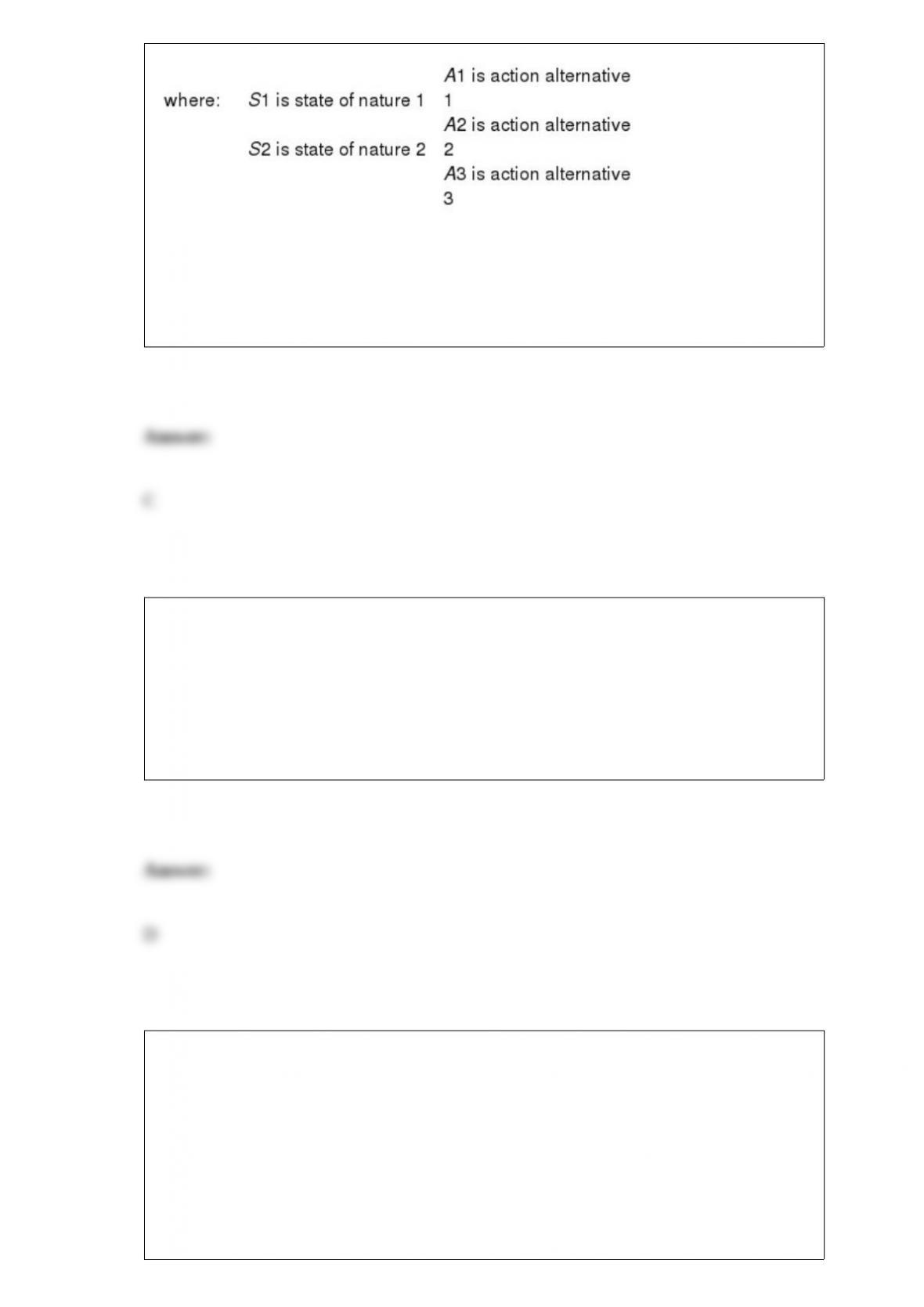
Referring to Table 19-1, if the probability of S1 is 0.4, then the probability of S2 is
A) 0.4.
B) 0.5.
C) 0.6.
D) 1.0.
A Paso Robles wine producer wanted to forecast the cases of Merlot wine sold. The
number of cases of merlot wine sold in a 28-year period was collected. Which of the
following would be the most appropriate analysis to perform?
A) The Marascuilo Procedure
B) The Tukey-Kramer Procedure
C) Least-squares forecasting with monthly or quarterly data
D) Exponential smoothing modeling
A statistics student found a reference in the campus library that contained the median
family incomes for all 50 states. She would report her data as being collected using
A) a designed experiment.
B) observational data.
C) a random sample.
D) a published source.
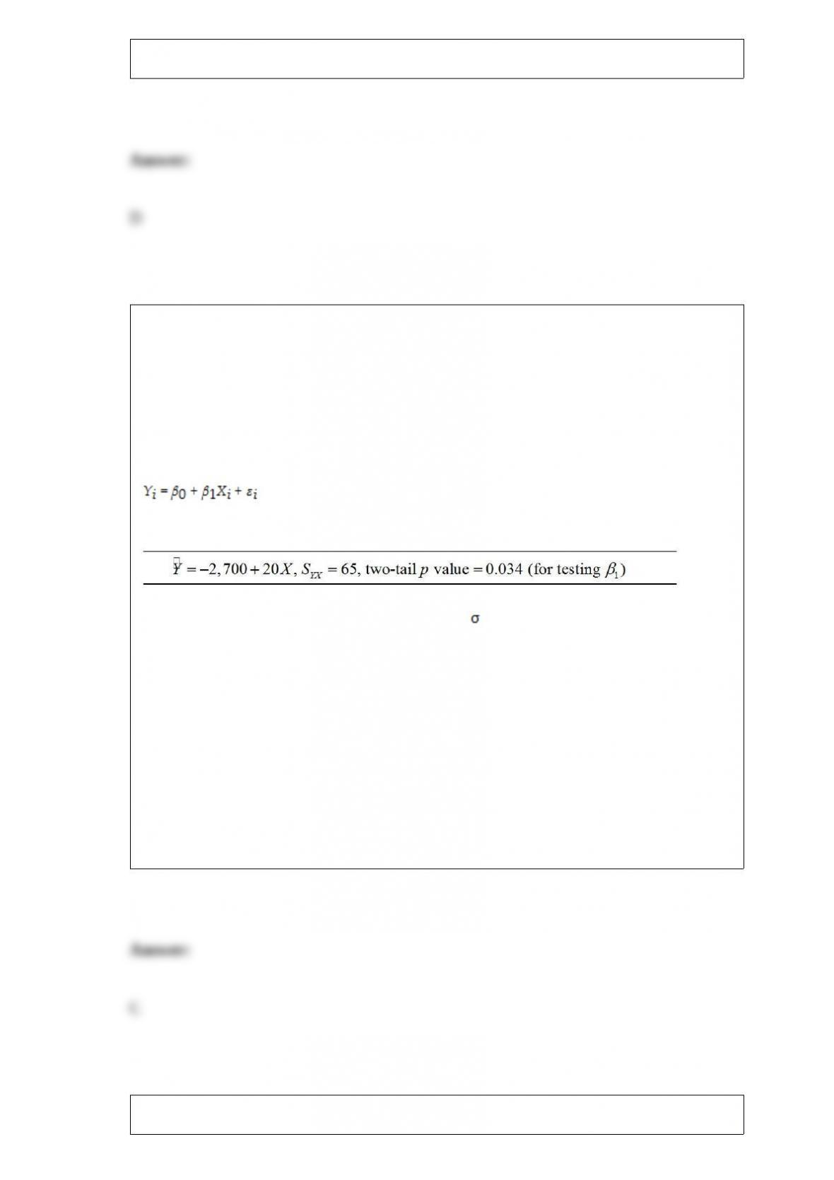
TABLE 13-1
A large national bank charges local companies for using their services. A bank official
reported the results of a regression analysis designed to predict the bank’s charges (Y) –
measured in dollars per month – for services rendered to local companies. One
independent variable used to predict service charges to a company is the company’s
sales revenue (X) – measured in millions of dollars. Data for 21 companies who use the
bank’s services were used to fit the model:
The results of the simple linear regression are provided below.
Referring to Table 13-1, interpret the estimate of , the standard deviation of the
random error term (standard error of the estimate) in the model.
A) About 95% of the observed service charges fall within $65 of the least squares line.
B) About 95% of the observed service charges equal their corresponding predicted
values.
C) About 95% of the observed service charges fall within $130 of the least squares line.
D) For every $1 million increase in sales revenue, we expect a service charge to
increase $65.
TABLE 13-12
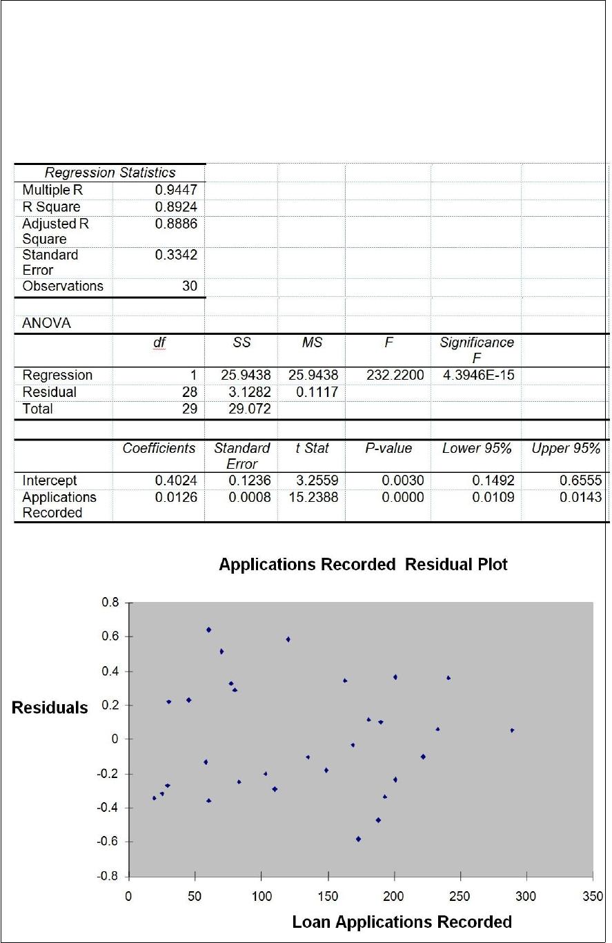
The manager of the purchasing department of a large saving and loan organization
would like to develop a model to predict the amount of time (measured in hours) it
takes to record a loan application. Data are collected from a sample of 30 days, and the
number of applications recorded and completion time in hours is recorded. Below is the
regression output:
Referring to Table 13-12, the error sum of squares (SSE) of the above regression is
A) 0.1117.
B) 3.1282.
C) 25.9438.
D) 29.0720.
If you were constructing a 99% confidence interval of the population mean based on a
sample of n = 25 where the standard deviation of the sample S = 0.05, the critical value
of t will be
A) 2.7969.
B) 2.7874.
C) 2.4922.
D) 2.4851.

If two events are mutually exclusive and collectively exhaustive, what is the probability
that both occur?
A) 0
B) 0.50
C) 1.00
D) Cannot be determined from the information given.
It is possible to directly compare the results of a confidence interval estimate to the
results obtained by testing a null hypothesis if
A) a two-tail test for is used.
B) a one-tail test for is used.
C) Both of the previous statements are true.
D) None of the previous statements is true.
TABLE 17-2
One of the most common questions of prospective house buyers pertains to the cost of
heating in dollars (Y). To provide its customers with information on that matter, a large
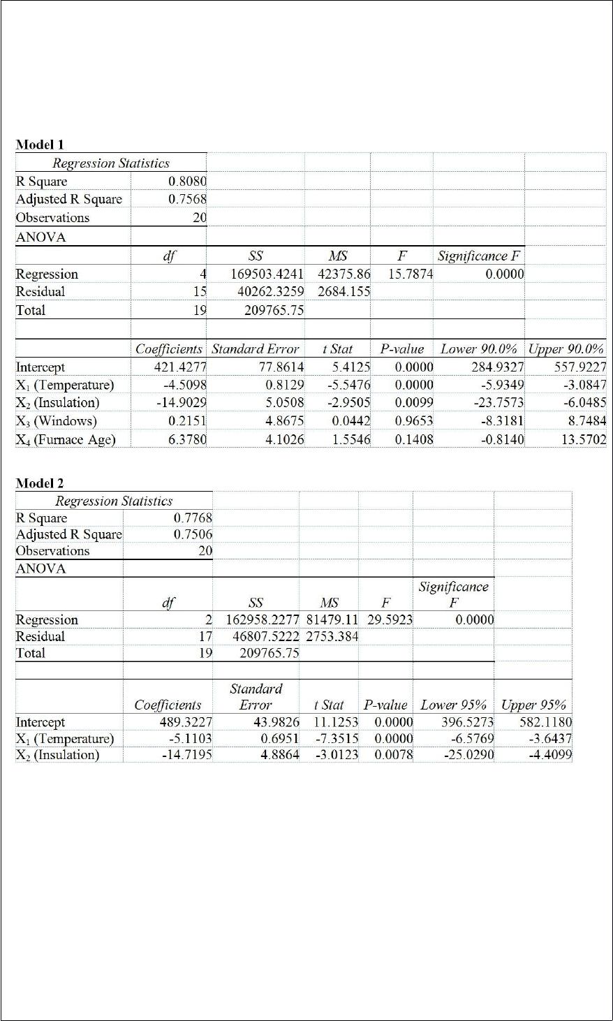
real estate firm used the following 4 variables to predict heating costs: the daily
minimum outside temperature in degrees of Fahrenheit (X1), the amount of insulation in
inches (X2), the number of windows in the house (X3), and the age of the furnace in
years (X4). Given below are the EXCEL outputs of two regression models.
Referring to Table 17-2, what is your decision and conclusion for the test H0 : β2 = 0
vs. H1 : β2 < 0 at the α = 0.01 level of significance using Model 1?
A) Do not reject H0 and conclude that the amount of insulation has a linear effect on
heating cots.
B) Reject H0 and conclude that the amount of insulation does not have a linear effect on
heating costs.
C) Reject H0 and conclude that the amount of insulation has a negative linear effect on
heating costs.
D) Do not reject H0 and conclude that the amount of insulation has a negative linear
effect on heating costs.
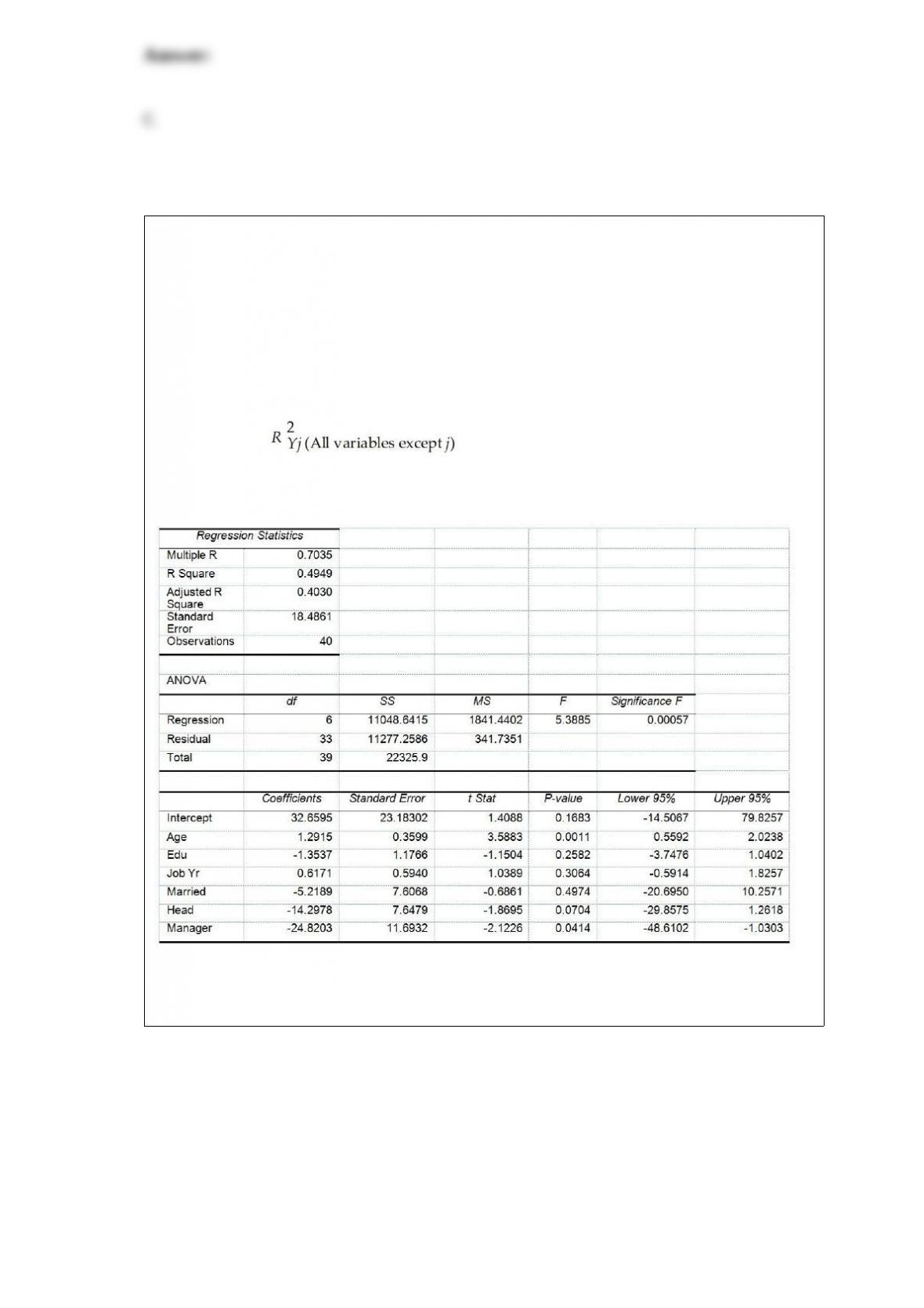
TABLE 17-10
Given below are results from the regression analysis where the dependent variable is
the number of weeks a worker is unemployed due to a layoff (Unemploy) and the
independent variables are the age of the worker (Age), the number of years of education
received (Edu), the number of years at the previous job (Job Yr), a dummy variable for
marital status (Married: 1 = married, 0 = otherwise), a dummy variable for head of
household (Head: 1 = yes, 0 = no) and a dummy variable for management position
(Manager: 1 = yes, 0 = no). We shall call this Model 1. The coefficient of partial
determination ( ) of each of the 6 predictors are, respectively,
0.2807, 0.0386, 0.0317, 0.0141, 0.0958, and 0.1201.
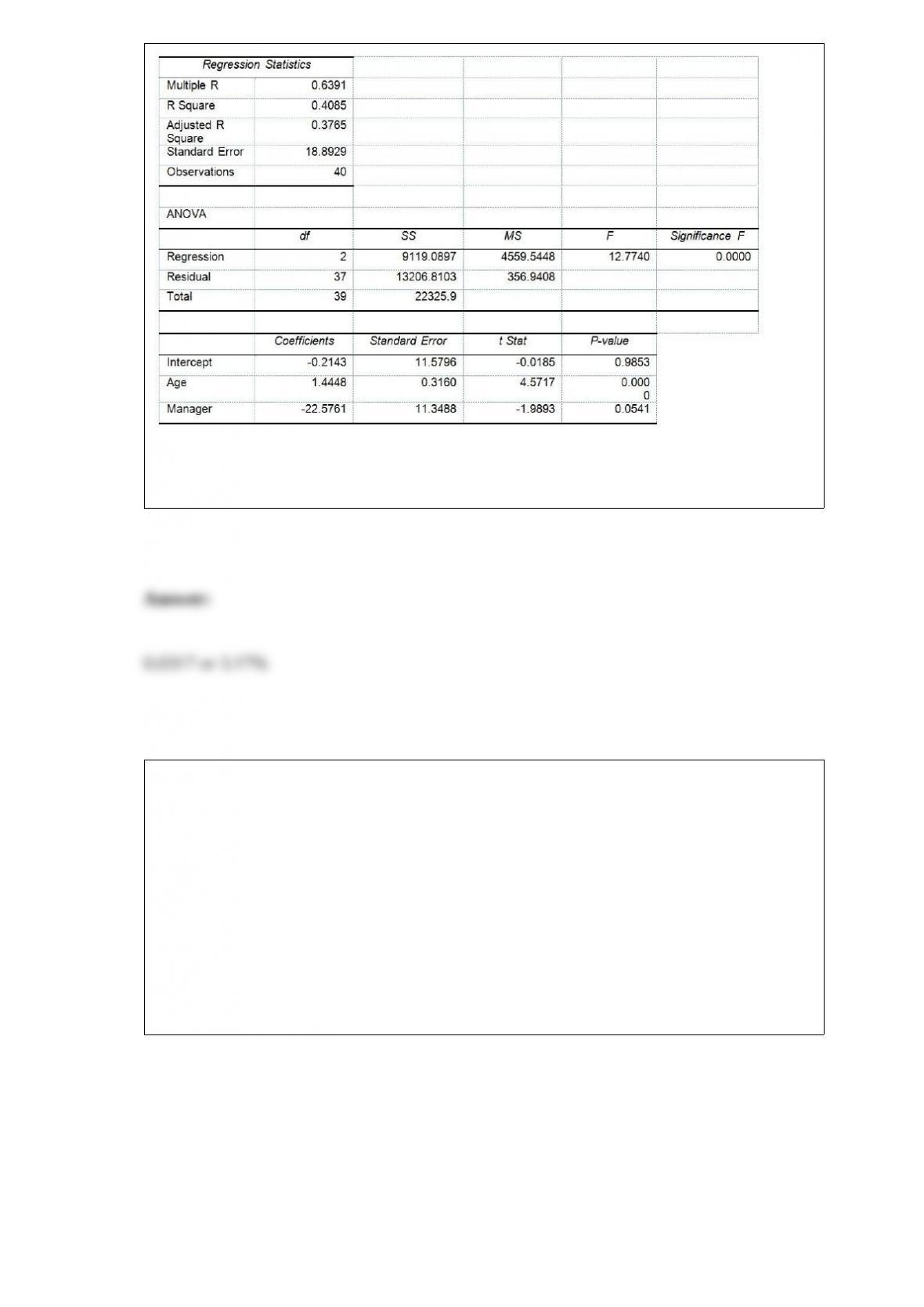
Model 2 is the regression analysis where the dependent variable is Unemploy and the
independent variables are Age and Manager. The results of the regression analysis are
given below:
Referring to Table 17-10, Model 1, ________ of the variation in the number of weeks a
worker is unemployed due to a layoff can be explained by the number of years at the
previous job while controlling for the other independent variables.
TABLE 17-12
The marketing manager for a nationally franchised lawn service company would like to
study the characteristics that differentiate home owners who do and do not have a lawn
service. A random sample of 30 home owners located in a suburban area near a large
city was selected; 15 did not have a lawn service (code 0) and 15 had a lawn service
(code 1). Additional information available concerning these 30 home owners includes
family income (Income, in thousands of dollars), lawn size (Lawn Size, in thousands of
square feet), attitude toward outdoor recreational activities (Attitude 0 = unfavorable, 1
= favorable), number of teenagers in the household (Teenager), and age of the head of
the household (Age).
The Minitab output is given below:
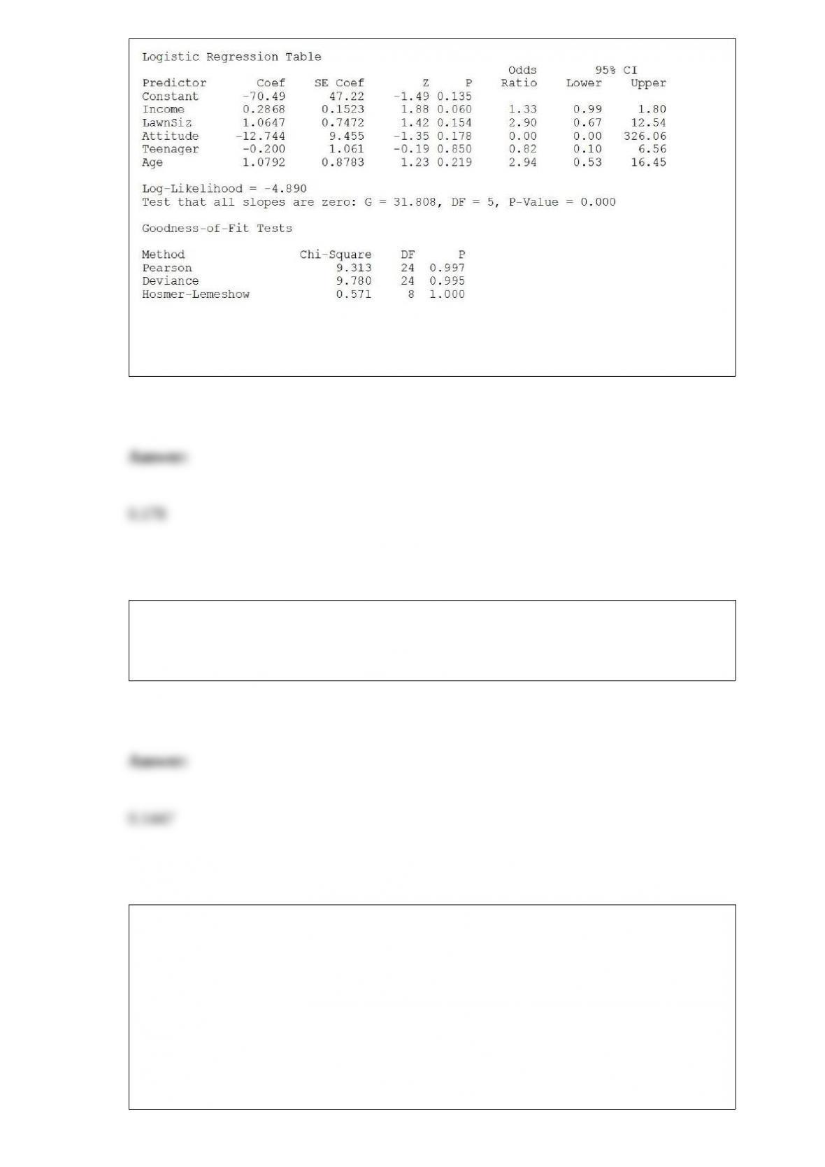
Referring to Table 17-12, what is the p-value of the test statistic when testing whether
Attitude makes a significant contribution to the model in the presence of the other
independent variables?
The amount of time between successive TV watching by first graders follows an
exponential distribution with a mean of 10 hours. The probability that a given first
grader spends between 10 and 15 hours between successive TV watching is ________.
TABLE 17-10
Given below are results from the regression analysis where the dependent variable is
the number of weeks a worker is unemployed due to a layoff (Unemploy) and the
independent variables are the age of the worker (Age), the number of years of education
received (Edu), the number of years at the previous job (Job Yr), a dummy variable for
marital status (Married: 1 = married, 0 = otherwise), a dummy variable for head of
household (Head: 1 = yes, 0 = no) and a dummy variable for management position
(Manager: 1 = yes, 0 = no). We shall call this Model 1. The coefficient of partial
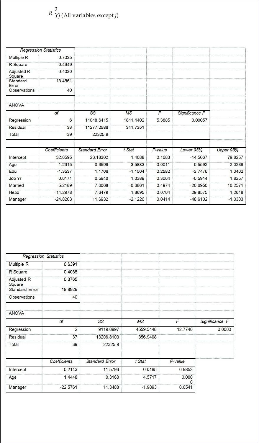
determination ( ) of each of the 6 predictors are, respectively,
0.2807, 0.0386, 0.0317, 0.0141, 0.0958, and 0.1201.
Model 2 is the regression analysis where the dependent variable is Unemploy and the
independent variables are Age and Manager. The results of the regression analysis are
given below:
Referring to Table 17-10, Model 1, what are the lower and upper limits of the 95%
confidence interval estimate for the difference in the mean number of weeks a worker is
unemployed due to a layoff between a worker who is married and one who is not after
taking into consideration the effect of all the other independent variables?
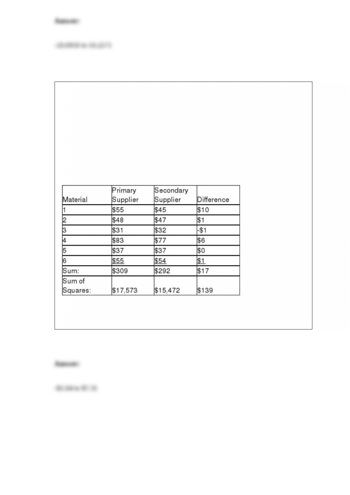
TABLE 10-7
A buyer for a manufacturing plant suspects that his primary supplier of raw materials is
overcharging. In order to determine if his suspicion is correct, he contacts a second
supplier and asks for the prices on various identical materials. He wants to compare
these prices with those of his primary supplier. The data collected is presented in the
table below, with some summary statistics presented (all of these might not be
necessary to answer the questions which follow). The buyer believes that the
differences are normally distributed and will use this sample to perform an appropriate
test at a level of significance of 0.01.
Referring to Table 10-7, what is the 95% confidence interval estimate for the mean
difference in prices?