
True or False: If the covariance between two investments is zero, the variance of the
sum of the two investments will be equal to the sum of the variances of the investments.
True or False: As a general rule, a value is considered an extreme value if its Z score is
less than 3.
TABLE 8-10
A sales and marketing management magazine conducted a survey on salespeople
cheating on their expense reports and other unethical conduct. In the survey on 200
managers, 58% of the managers have caught salespeople cheating on an expense report,
50% have caught salespeople working a second job on company time, 22% have caught
salespeople listing a ‘strip bar” as a restaurant on an expense report, and 19% have
caught salespeople giving a kickback to a customer.
True or False: Referring to Table 8-10, a 95% confidence interval will contain 95% of
the population proportion of managers who have caught salespeople cheating on an
expense report.

TABLE 11-11
A student team in a business statistics course designed an experiment to investigate
whether the brand of bubblegum used affected the size of bubbles they could blow. To
reduce the person-to-person variability, the students decided to use a randomized block
design using themselves as blocks.
Four brands of bubblegum were tested. A student chewed two pieces of a brand of gum
and then blew a bubble, attempting to make it as big as possible. Another student
measured the diameter of the bubble at its biggest point. The following table gives the
diameters of the bubbles (in inches) for the 16 observations.
True or False: Referring to Table 11-11, the null hypothesis for the F test for the block
effects should be rejected at a 0.05 level of significance.
TABLE 8-7
A hotel chain wants to estimate the mean number of rooms rented daily in a given
month. The population of rooms rented daily is assumed to be normally distributed for
each month with a standard deviation of 240 rooms. During February, a sample of 25
days has a sample mean of 370 rooms.
True or False: Referring to Table 8-7, a 99% confidence interval will contain 99% of the
sample mean number of rooms rented daily in a given month.
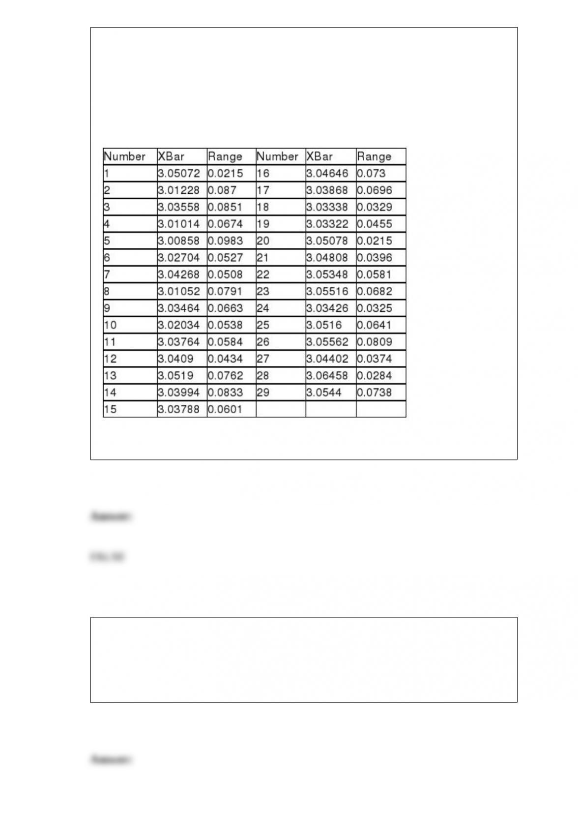
True or False: TABLE 18-9
The manufacturer of canned food constructed control charts and analyzed several
quality characteristics. One characteristic of interest is the weight of the filled cans. The
lower specification limit for weight is 2.95 pounds. The table below provides the range
and mean of the weights of five cans tested every fifteen minutes during a day’s
production.
Referring to Table 18-9, based on the R chart, it appears that the process is out of
control.
True or False: A sample is used to obtain a 95% confidence interval for the mean of a
population. The confidence interval goes from 15 to 19. If the same sample had been
used to test the null hypothesis that the mean of the population is equal to 18 versus the
alternative hypothesis that the mean of the population differs from 18, the null
hypothesis could be rejected at a level of significance of 0.05.
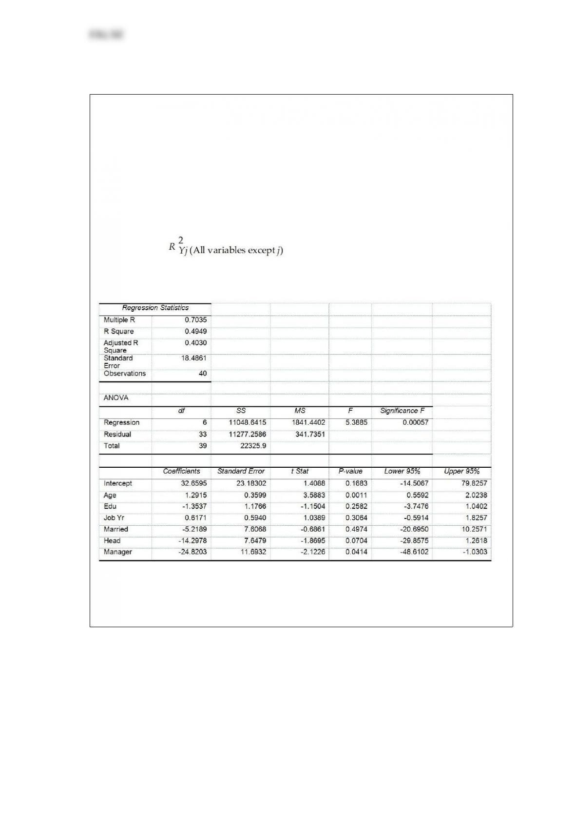
True or False: TABLE 17-10
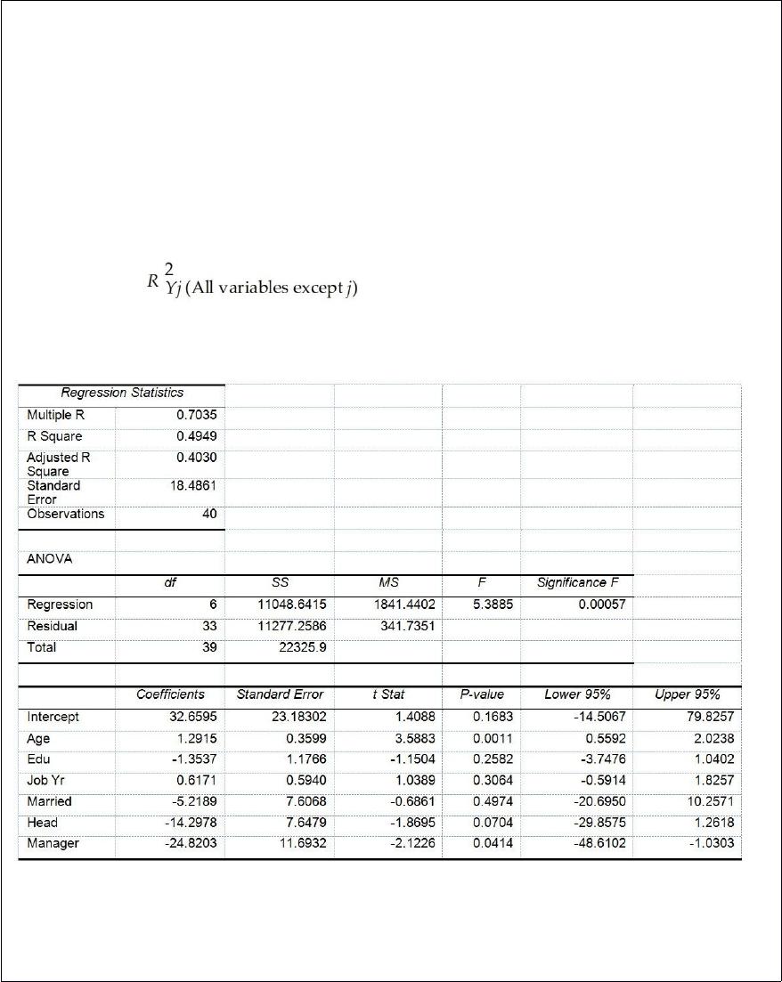
Given below are results from the regression analysis where the dependent variable is
the number of weeks a worker is unemployed due to a layoff (Unemploy) and the
independent variables are the age of the worker (Age), the number of years of education
received (Edu), the number of years at the previous job (Job Yr), a dummy variable for
marital status (Married: 1 = married, 0 = otherwise), a dummy variable for head of
household (Head: 1 = yes, 0 = no) and a dummy variable for management position
(Manager: 1 = yes, 0 = no). We shall call this Model 1. The coefficient of partial
determination ( ) of each of the 6 predictors are, respectively,
0.2807, 0.0386, 0.0317, 0.0141, 0.0958, and 0.1201.
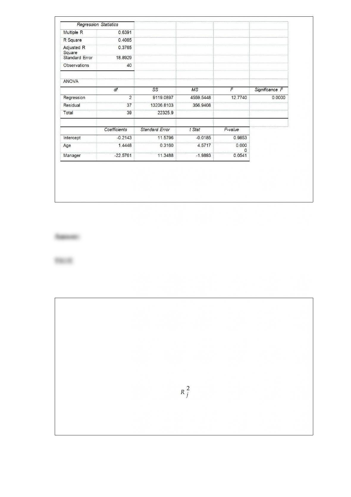
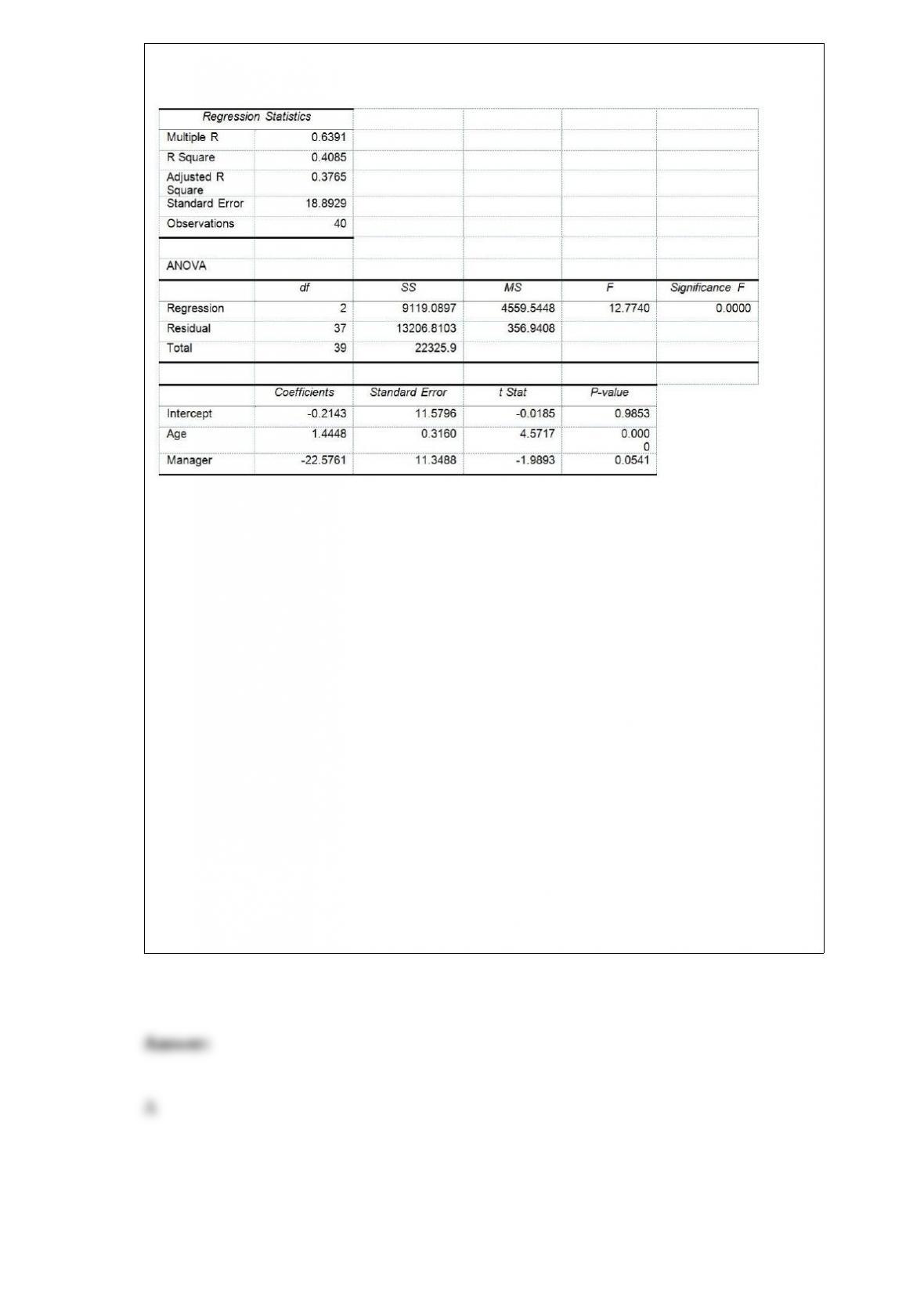
Model 2 is the regression analysis where the dependent variable is Unemploy and the
independent variables are Age and Manager. The results of the regression analysis are
given below:
Referring to Table 17-10, Model 1, the null hypothesis should be rejected at a 10% level
of significance when testing whether age has any effect on the number of weeks a
worker is unemployed due to a layoff.
TABLE 15-6
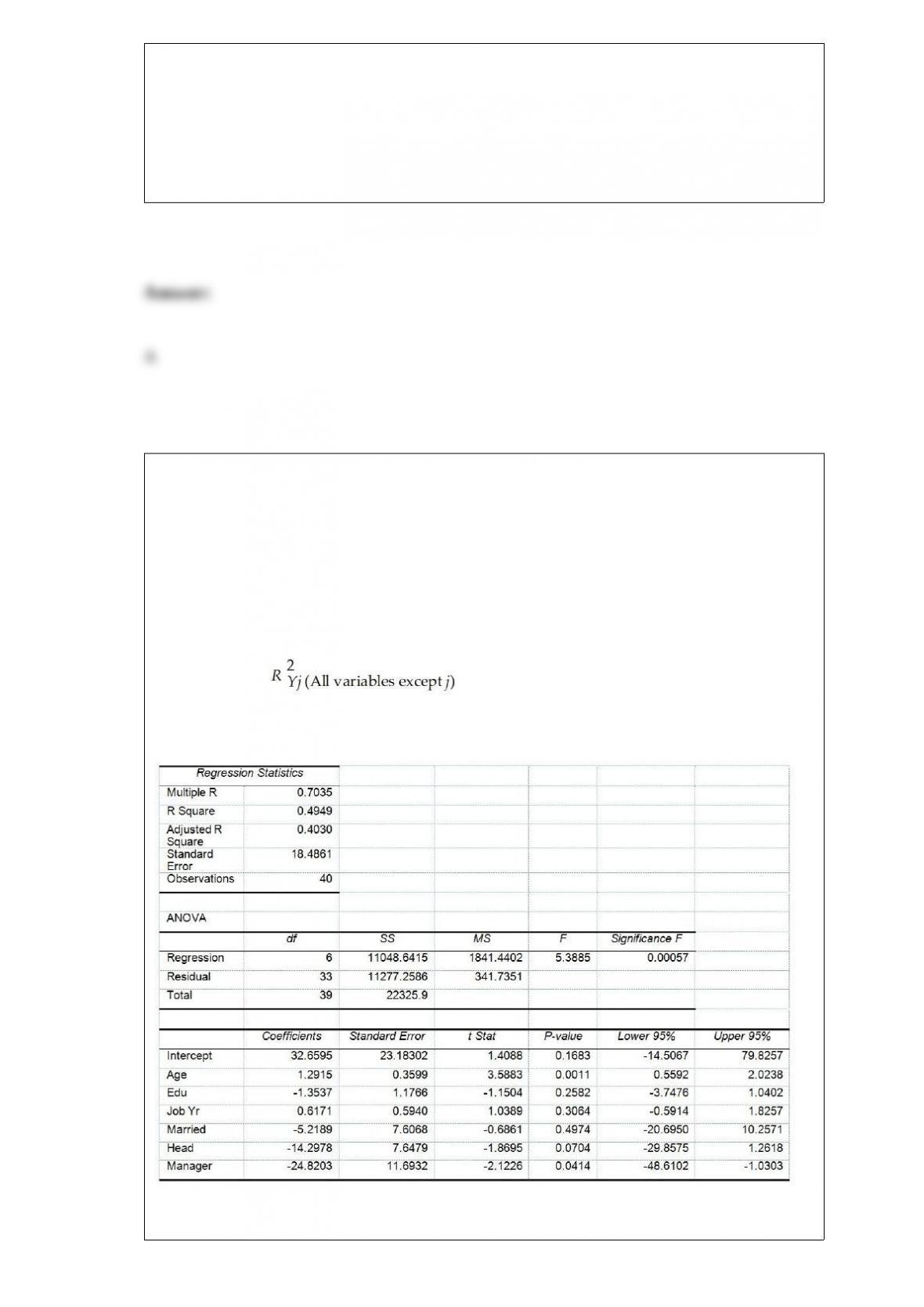
Given below are results from the regression analysis on 40 observations where the
dependent variable is the number of weeks a worker is unemployed due to a layoff (Y)
and the independent variables are the age of the worker (X1), the number of years of
education received (X2), the number of years at the previous job (X3), a dummy variable
for marital status (X4: 1 = married, 0 = otherwise), a dummy variable for head of
household (X5: 1 = yes, 0 = no) and a dummy variable for management position (X6: 1
= yes, 0 = no).
The coefficient of multiple determination ( ) for the regression model using each of
the 6 variables Xj as the dependent variable and all other X variables as independent
variables are, respectively, 0.2628, 0.1240, 0.2404, 0.3510, 0.3342 and 0.0993.
The partial results from best-subset regression are given below:
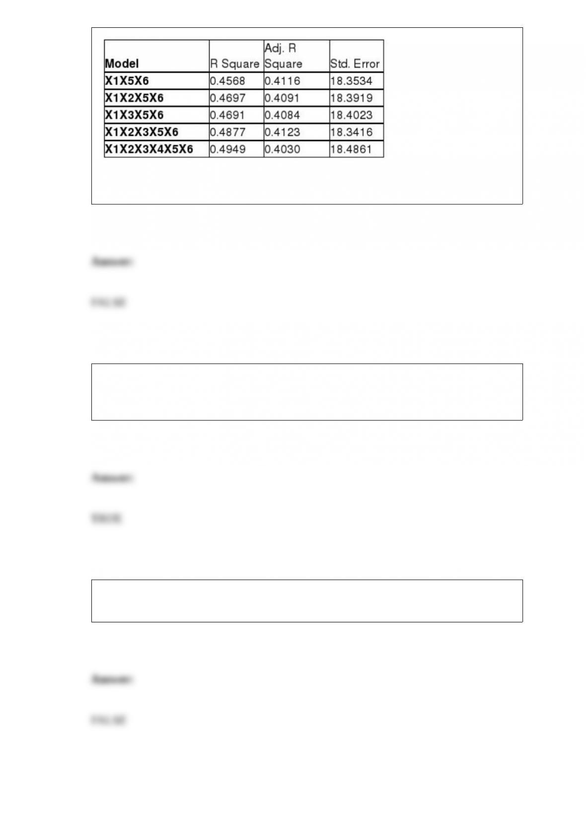
True or False: Referring to Table 15-6, the variable X1 should be dropped to remove
collinearity.
True or False: Business analytics combine “traditional” statistical methods with
methods and techniques from management science and information systems to form an
interdisciplinary tool that supports fact-based management decision making.
True or False: If remains constant in a binomial distribution, an increase in n will not
change the mean.
True or False: TABLE 17-10
Given below are results from the regression analysis where the dependent variable is
the number of weeks a worker is unemployed due to a layoff (Unemploy) and the
independent variables are the age of the worker (Age), the number of years of education
received (Edu), the number of years at the previous job (Job Yr), a dummy variable for
marital status (Married: 1 = married, 0 = otherwise), a dummy variable for head of
household (Head: 1 = yes, 0 = no) and a dummy variable for management position
(Manager: 1 = yes, 0 = no). We shall call this Model 1. The coefficient of partial
determination ( ) of each of the 6 predictors are, respectively,
0.2807, 0.0386, 0.0317, 0.0141, 0.0958, and 0.1201.
Model 2 is the regression analysis where the dependent variable is Unemploy and the
independent variables are Age and Manager. The results of the regression analysis are
given below:
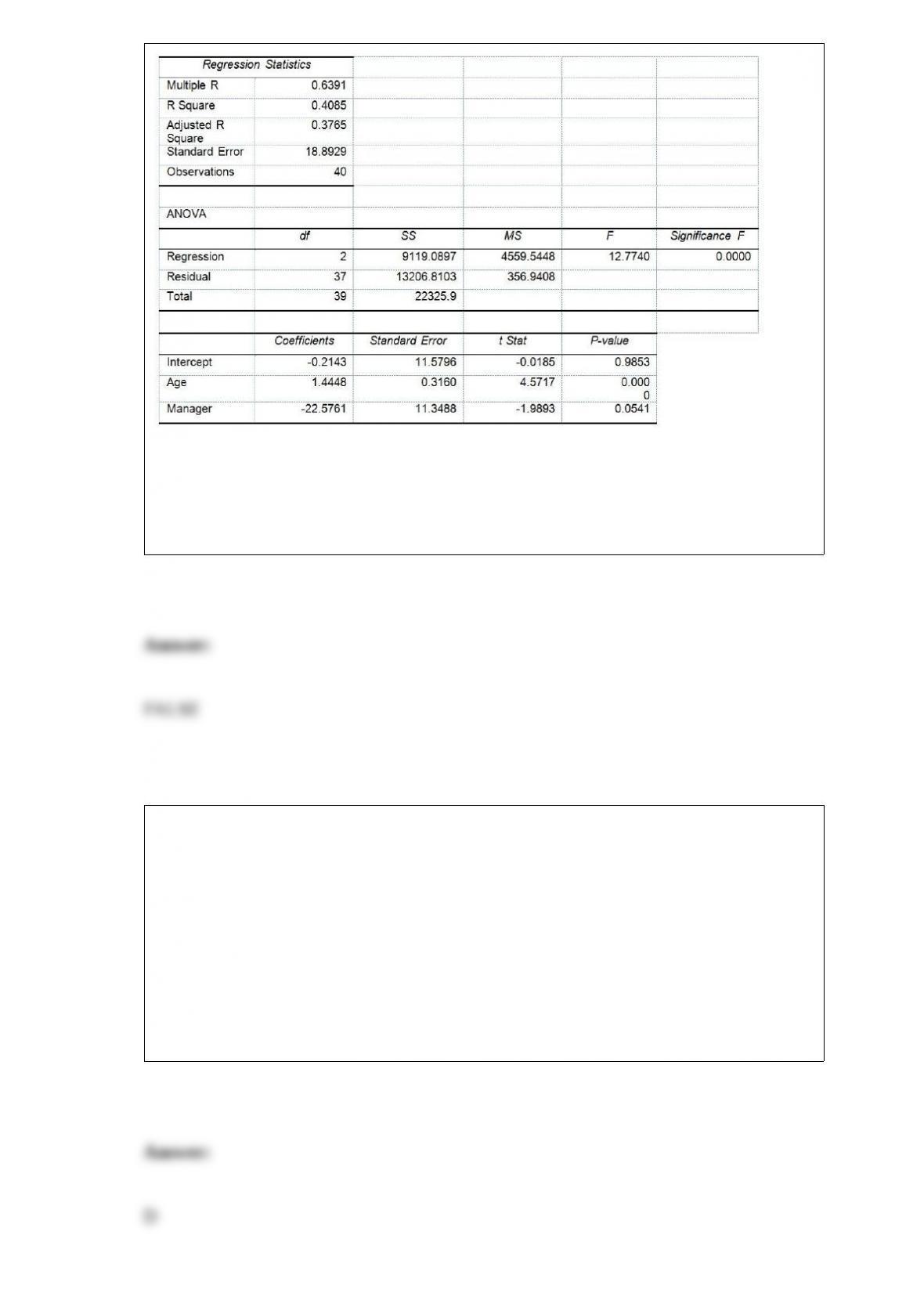
Referring to Table 17-10 and using both Model 1 and Model 2, there is sufficient
evidence to conclude that the independent variables that are not significant individually
are also not significant as a group in explaining the variation in the dependent variable
at a 5% level of significance.
The power of a statistical test is
A) the probability of not rejecting H0 when it is false.
B) the probability of rejecting H0 when it is true.
C) the probability of not rejecting H0 when it is true.
D) the probability of rejecting H0 when it is false.
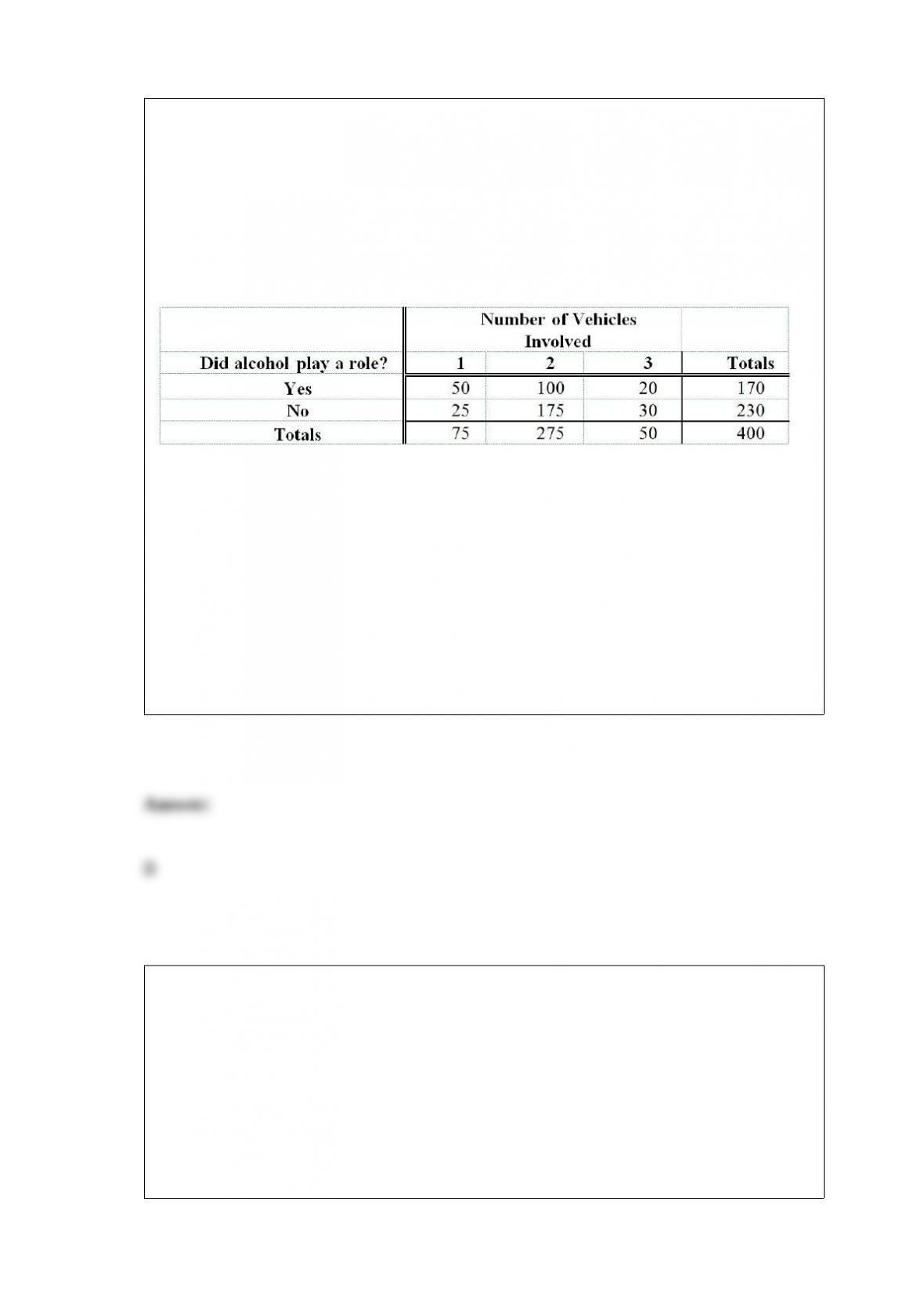
TABLE 4-1
Mothers Against Drunk Driving is a very visible group whose main focus is to educate
the public about the harm caused by drunk drivers. A study was recently done that
emphasized the problem we all face with drinking and driving. Four hundred accidents
that occurred on a Saturday night were analyzed. Two items noted were the number of
vehicles involved and whether alcohol played a role in the accident. The numbers are
shown below:
Referring to Table 4-1, given that 3 vehicles were involved, what proportion of
accidents involved alcohol?
A) 20/30 or 66.67%
B) 20/50 or 40%
C) 20/170 or 11.77%
D) 20/400 or 5%
Which of the following is sensitive to extreme values?
A) the median
B) the interquartile range
C) the arithmetic mean
D) the 1st quartile

If you know that the level of significance ( ) of a test is 5%, you can tell that the
probability of committing a Type II error ( ) is
A) 2.5%.
B) 95%.
C) 97.5%.
D) unknown.
TABLE 13-9
It is believed that, the average numbers of hours spent studying per day (HOURS)
during undergraduate education should have a positive linear relationship with the
starting salary (SALARY, measured in thousands of dollars per month) after graduation.
Given below is the Excel output for predicting starting salary (Y) using number of hours
spent studying per day (X) for a sample of 51 students. NOTE: Only partial output is
shown.
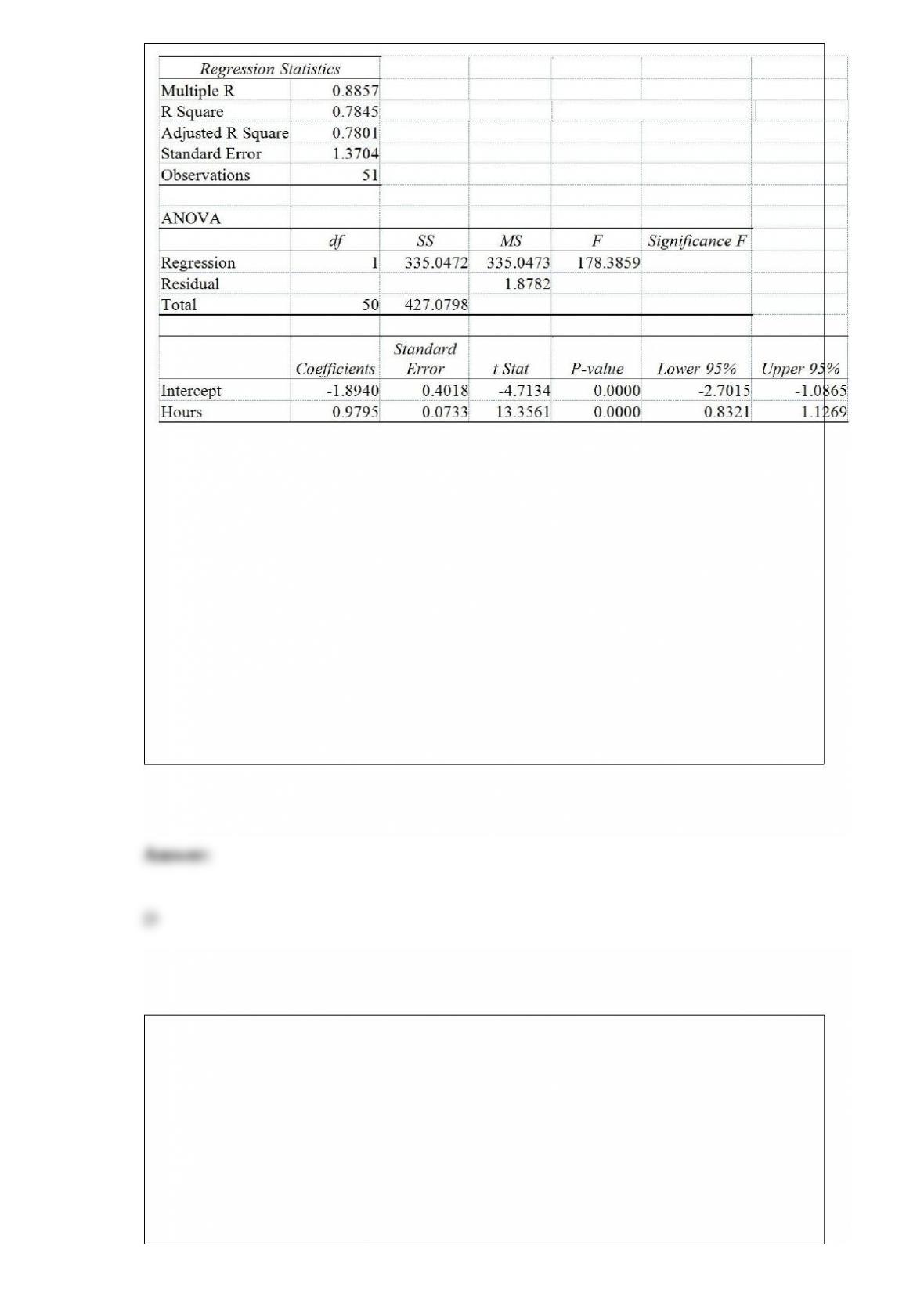
Note: 2.051E – 05 = 2.051 ∗ 10-05 and 5.944E – 18 = 5.944 ∗ 10-18.
Referring to Table 13-9, the 90% confidence interval for the average change in
SALARY (in thousands of dollars) as a result of spending an extra hour per day
studying is
A) wider than [-2.70159, -1.08654].
B) narrower than [-2.70159, -1.08654].
C) wider than [0.8321927, 1.12697].
D) narrower than [0.8321927, 1.12697].
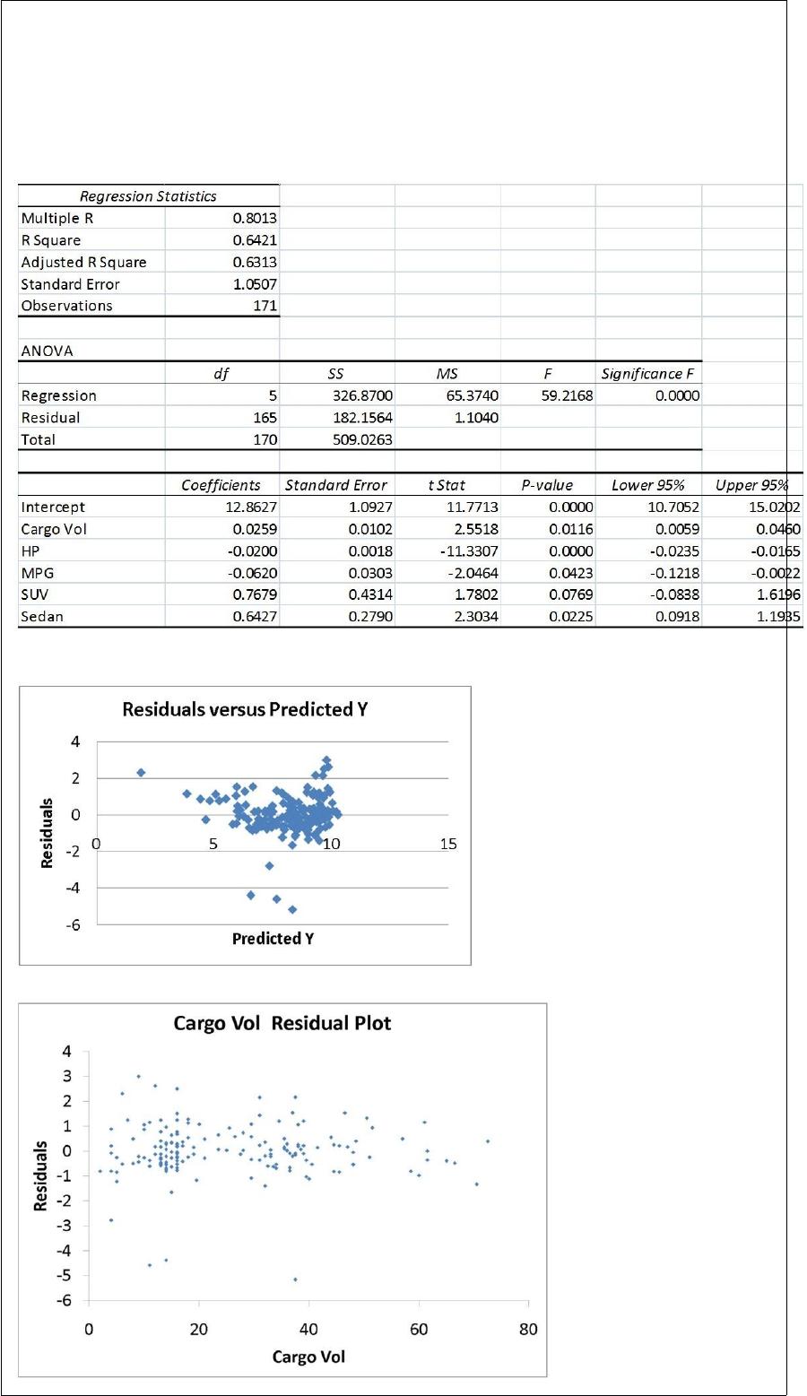
TABLE 17-9
What are the factors that determine the acceleration time (in sec.) from 0 to 60 miles per
hour of a car? Data on the following variables for 171 different vehicle models were
collected:
Accel Time: Acceleration time in sec.
Cargo Vol: Cargo volume in cu. ft.
HP: Horsepower
MPG: Miles per gallon
SUV: 1 if the vehicle model is an SUV with Coupe as the base when SUV and Sedan
are both 0
Sedan: 1 if the vehicle model is a sedan with Coupe as the base when SUV and Sedan
are both 0
The regression results using acceleration time as the dependent variable and the
remaining variables as the independent variables are presented below.
The various residual plots are as shown below.
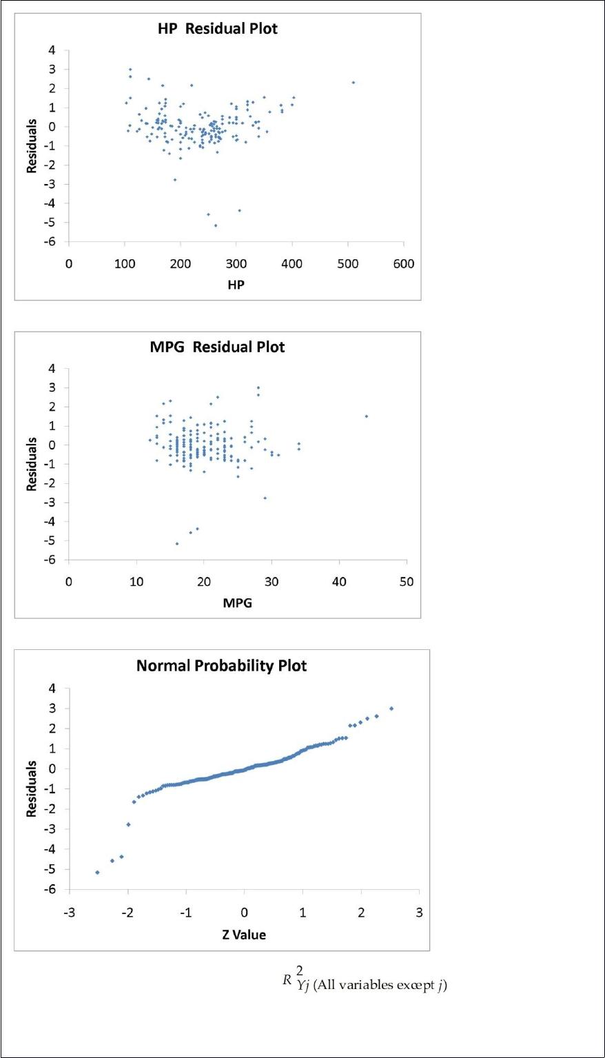
The coefficient of partial determination ( ) of each of the 5
predictors are, respectively, 0.0380, 0.4376, 0.0248, 0.0188, and 0.0312.
The coefficient of multiple determination for the regression model using each of the 5
variables Xj as the dependent variable and all other X variables as independent variables
( ) are, respectively, 0.7461, 0.5676, 0.6764, 0.8582, 0.6632.
Referring to Table 17-9, what is the correct interpretation for the estimated coefficient
for Cargo Vol?
A) As the 0 to 60 miles per hour acceleration time increases by one second, the mean
cargo volume will increase by an estimated 0.0259 cubic foot without taking into
consideration all the other independent variables included in the model.
B) As the cargo volume increases by one cubic foot, the mean 0 to 60 miles per hour
acceleration time will increase by an estimated 0.0259 seconds without taking into
consideration all the other independent variables included in the model.
C) As the 0 to 60 miles per hour acceleration time increases by one second, the mean
cargo volume will increase by an estimated 0.0259 cubic foot taking into consideration
all the other independent variables included in the model.
D) As the cargo volume increases by one cubic foot, the mean 0 to 60 miles per hour
acceleration time will increase by an estimated 0.0259 seconds taking into
consideration all the other independent variables included in the model.
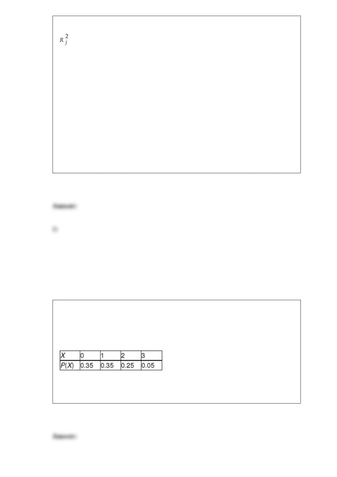
TABLE 5-3
The following table contains the probability distribution for X = the number of
retransmissions necessary to successfully transmit a 1024K data package through a
double satellite media.
Referring to Table 5-3, the mean or expected value for the number of retransmissions is
________.

TABLE 7-2
The mean selling price of new homes in a small town over a year was $115,000. The
population standard deviation was $25,000. A random sample of 100 new home sales
from this city was taken.
Referring to Table 7-2, without doing the calculations, state in which of the following
ranges the sample mean selling price is most likely to lie.
A) $113,000-$115,000
B) $114,000-$116,000
C) $115,000-$117,000
D) $116,000-$118,000
A population frame for a survey contains a listing of 6,179 names. Using a table of
random numbers, which of the following code numbers will appear on your list?
A) 06
B) 0694
C) 6946
D) 61790
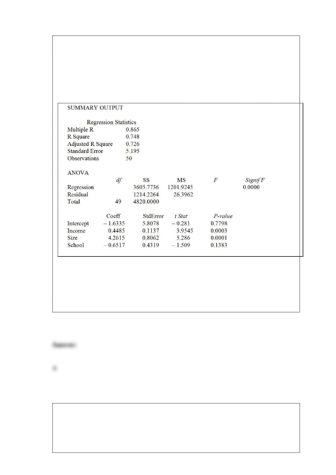
TABLE 17-1
A real estate builder wishes to determine how house size (House) is influenced by
family income (Income), family size (Size), and education of the head of household
(School). House size is measured in hundreds of square feet, income is measured in
thousands of dollars, and education is in years. The builder randomly selected 50
families and ran the multiple regression. Microsoft Excel output is provided below:
Referring to Table 17-1, what are the regression degrees of freedom that are missing
from the output?
A) 3
B) 46
C) 49
D) 50
An Undergraduate Study Committee of 6 members at a major university is to be formed
from a pool of faculty of 18 men and 6 women. Which of the following distributions
would you use to determine the probability that half of the members will be women?
A) Hypergeometric distribution
B) Poisson distribution
C) Uniform distribution
D) Binomial distribution
TABLE 17-10
Given below are results from the regression analysis where the dependent variable is
the number of weeks a worker is unemployed due to a layoff (Unemploy) and the
independent variables are the age of the worker (Age), the number of years of education
received (Edu), the number of years at the previous job (Job Yr), a dummy variable for
marital status (Married: 1 = married, 0 = otherwise), a dummy variable for head of
household (Head: 1 = yes, 0 = no) and a dummy variable for management position
(Manager: 1 = yes, 0 = no). We shall call this Model 1. The coefficient of partial
determination ( ) of each of the 6 predictors are, respectively,
0.2807, 0.0386, 0.0317, 0.0141, 0.0958, and 0.1201.
Model 2 is the regression analysis where the dependent variable is Unemploy and the
independent variables are Age and Manager. The results of the regression analysis are
given below:
Referring to Table 17-10, Model 1, which of the following is a correct statement?
A) 49.49% of the total variation in the number of weeks a worker is unemployed due to
a layoff can be explained by the age of the worker, the number of years of education
received, the number of years at the previous job, marital status, whether the worker is
the head of household and whether the worker is a manager.
B) 49.49% of the total variation in the number of weeks a worker is unemployed due to
a layoff can be explained by the age of the worker, the number of years of education
received, the number of years at the previous job, marital status, whether the worker is
the head of household and whether the worker is a manager after adjusting for the
number of predictors and sample size.
C) 49.49% of the total variation in the number of weeks a worker is unemployed due to
a layoff can be explained by the age of the worker, the number of years of education
received, the number of years at the previous job, marital status, whether the worker is
the head of household and whether the worker is a manager after adjusting for the level
of significance.
D) 49.49% of the total variation in the number of weeks a worker is unemployed due to
a layoff can be explained by the age of the worker, the number of years of education
received, the number of years at the previous job, marital status, whether the worker is
the head of household and whether the worker is a manager holding constant the effect
of all the independent variables.
In purchasing an automobile, there are a number of variables to consider. The color of
the car is an example of a ________ variable.
TABLE 5-7
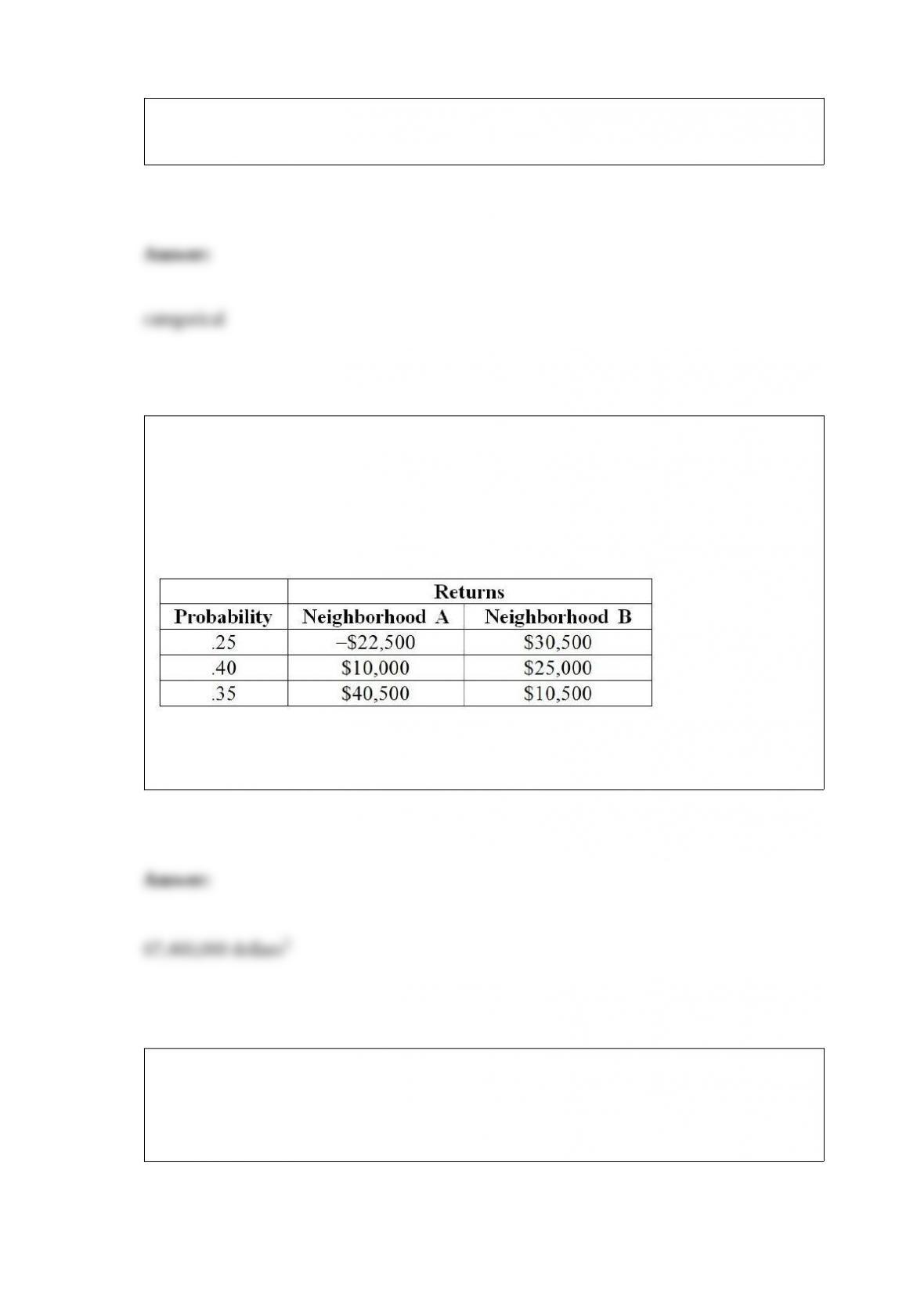
There are two houses with almost identical characteristics available for investment in
two different neighborhoods with drastically different demographic composition. The
anticipated gain in value when the houses are sold in 10 years has the following
probability distribution:
Referring to Table 5-7, what is the variance of the gain in value for the house in
neighborhood B?
TABLE 2-10
The histogram below represents scores achieved by 200 job applicants on a personality
profile.

Referring to the histogram from Table 2-10, half of the job applicants scored below
________.
TABLE 9-4
A drug company is considering marketing a new local anesthetic. The effective time of
the anesthetic the drug company is currently producing has a normal distribution with a
mean of 7.4 minutes with a standard deviation of 1.2 minutes. The chemistry of the new
anesthetic is such that the effective time should be normally distributed with the same
standard deviation, but the mean effective time may be lower. If it is lower, the drug
company will market the new anesthetic; otherwise, they will continue to produce the
older one. A sample size of 36 results in a sample mean of 7.1. A hypothesis test will be
done to help make the decision.
Referring to Table 9-4, for a test with a level of significance of 0.10, the critical value
would be ________.

The local police department must write, on average, 5 tickets a day to keep department
revenues at budgeted levels. Suppose the number of tickets written per day follows a
Poisson distribution with a mean of 6.4 tickets per day. Find the probability that exactly
6 tickets are written on a randomly selected day from this population.
TABLE 3-7
In a recent academic year, many public universities in the United States raised tuition
and fees due to a decrease in state subsidies. The change in the cost of tuition, a shared
dormitory room, and the most popular meal plan from the previous academic year for a
sample of 10 public universities were as follows: $1,589, $593, $1,223, $869, $423,
$1,720, $708, $1,425, $922 and $308.
Referring to Table 3-7, is the change in the cost lepokurtic or platykurtic?