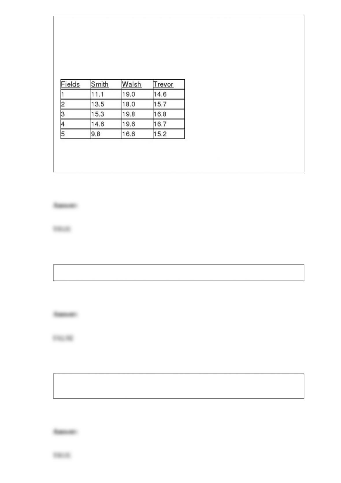
TABLE 11-10
An agronomist wants to compare the crop yield of 3 varieties of chickpea seeds. She
plants all 3 varieties of the seeds on each of 5 different patches of fields. She then
measures the crop yield in bushels per acre. Treating this as a randomized block design,
the results are presented in the table that follows.
True or False: Referring to Table 11-10, the randomized block F test is valid only if the
population of crop yields is normally distributed for the 3 varieties.
True or False: The consumer price index is a Paasche price index.
True or False: The Guidelines for Developing Visualizations recommend always
starting the scale for a vertical axis at zero.

True or False: The “middle spread,” that is the middle 50% of the normal distribution, is
equal to one standard deviation.
True or False: A zero population correlation coefficient between a pair of random
variables means that there is no linear relationship between the random variables.
True or False: The O in the DCOVA framework stands for “operationalize.”
True or False: A professor computed the sample average exam score of 20 students and
used it to estimate the average exam score of the 1,500 students taking the exam. This is
an example of inferential statistics.
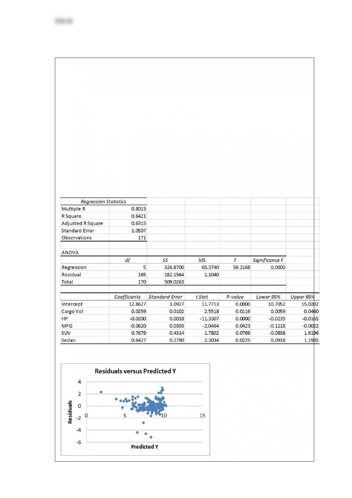
True or False: TABLE 17-9
What are the factors that determine the acceleration time (in sec.) from 0 to 60 miles per
hour of a car? Data on the following variables for 171 different vehicle models were
collected:
Accel Time: Acceleration time in sec.
Cargo Vol: Cargo volume in cu. ft.
HP: Horsepower
MPG: Miles per gallon
SUV: 1 if the vehicle model is an SUV with Coupe as the base when SUV and Sedan
are both 0
Sedan: 1 if the vehicle model is a sedan with Coupe as the base when SUV and Sedan
are both 0
The regression results using acceleration time as the dependent variable and the
remaining variables as the independent variables are presented below.
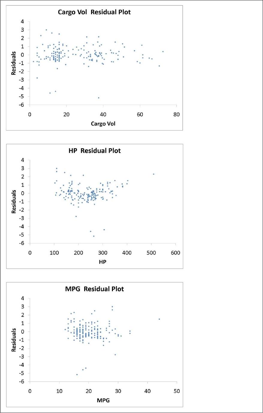
The various residual plots are as shown below.
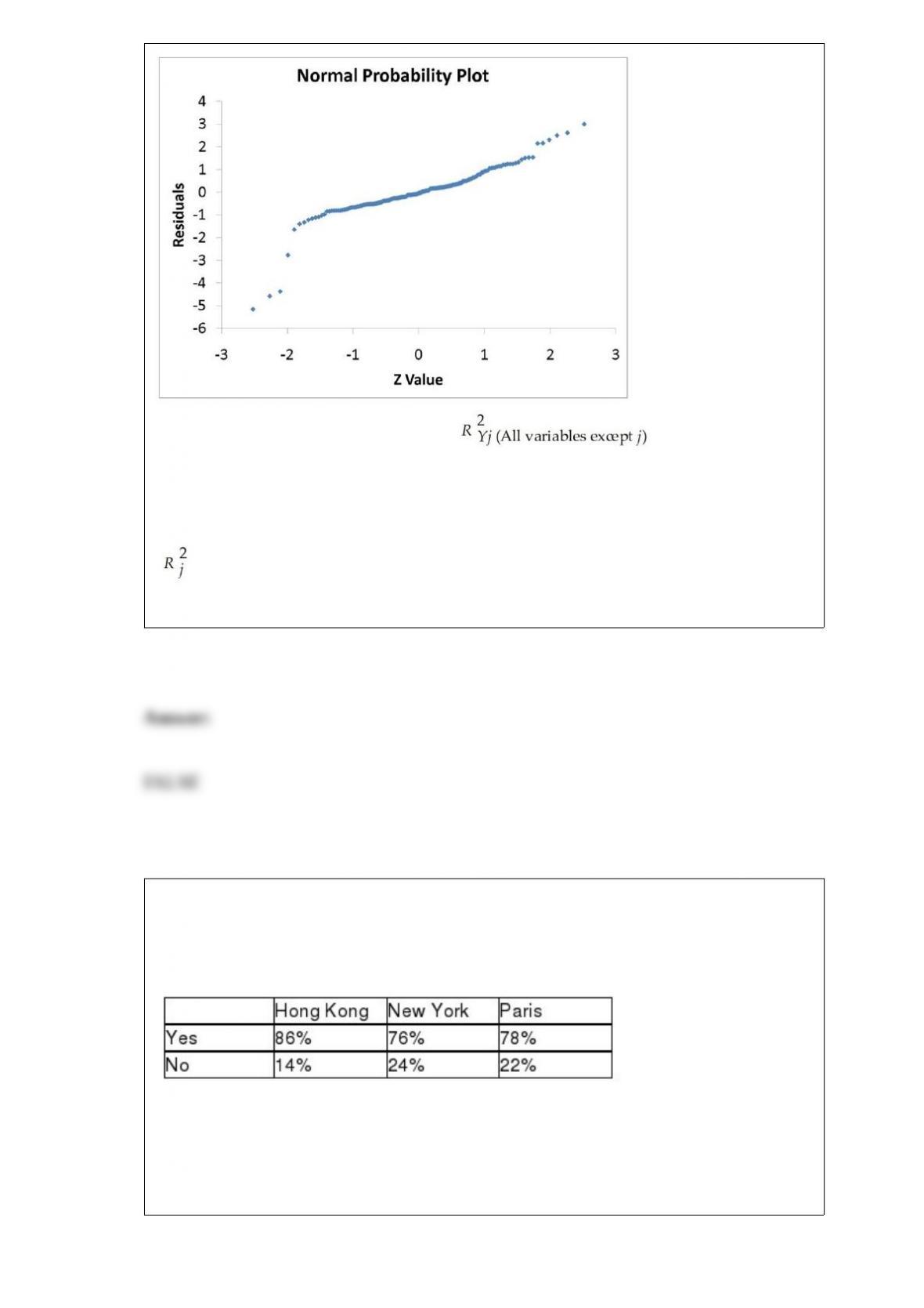
The coefficient of partial determination ( ) of each of the 5
predictors are, respectively, 0.0380, 0.4376, 0.0248, 0.0188, and 0.0312.
The coefficient of multiple determination for the regression model using each of the 5
variables Xj as the dependent variable and all other X variables as independent variables
( ) are, respectively, 0.7461, 0.5676, 0.6764, 0.8582, 0.6632.
Referring to Table 17-9, the errors (residuals) appear to be right-skewed.
TABLE 12-7
Data on the percentage of 200 hotels in each of the three large cities across the world on
whether minibar charges are correctly posted at checkout are given below.
At the 0.05 level of significance, you want to know if there is evidence of a difference
in the proportion of hotels that correctly post minibar charges among the three cities.
True or False: Referring to Table 12-7, the null hypothesis will be rejected.
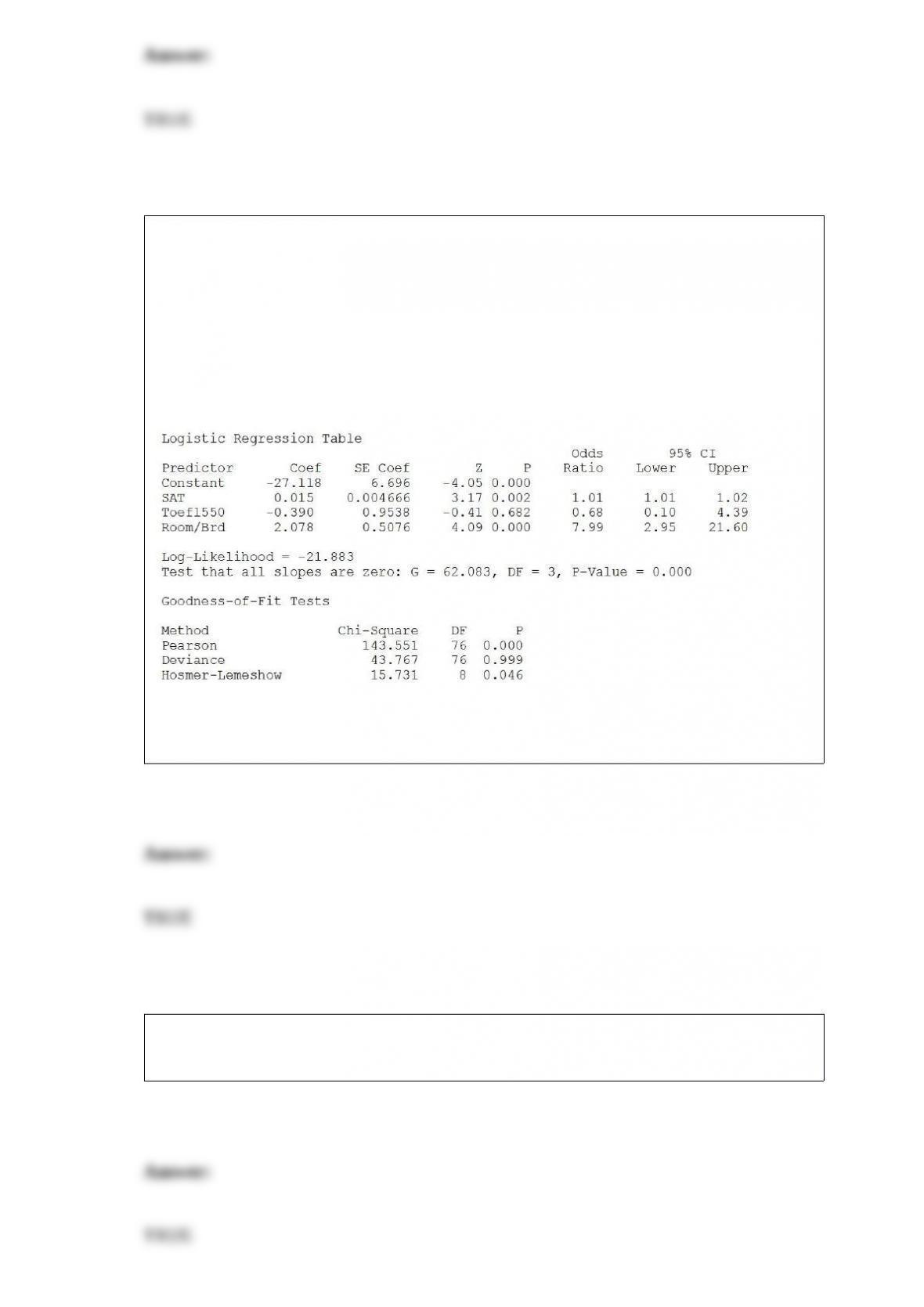
True or False: TABLE 17-11
A logistic regression model was estimated in order to predict the probability that a
randomly chosen university or college would be a private university using information
on mean total Scholastic Aptitude Test score (SAT) at the university or college, the
room and board expense measured in thousands of dollars (Room/Brd), and whether the
TOEFL criterion is at least 550 (Toefl550 = 1 if yes, 0 otherwise.) The dependent
variable, Y, is school type (Type = 1 if private and 0 otherwise).
Referring to Table 17-11, the null hypothesis that the model is a good-fitting model
cannot be rejected when allowing for a 5% probability of making a type I error.
True or False: A multiple regression is called “multiple” because it has several
explanatory variables.

TABLE 14-19
The marketing manager for a nationally franchised lawn service
company would like to study the characteristics that di erentiate
home owners who do and do not have a lawn service. A random
sample of 30 home owners located in a suburban area near a large
city was selected; 11 did not have a lawn service (code 0) and 19 had
a lawn service (code 1). Additional information available concerning
these 30 home owners includes family income (Income, in thousands
of dollars) and lawn size (Lawn Size, in thousands of square feet).
The PHStat output is given below:
True or False: Referring to Table 14-19, there is not enough evidence
to conclude that LawnSize makes a signiticant contribution to the
model in the presence of Income at a 0.05 level of signiticance.
TABLE 12-6
According to an article in Marketing News, fewer checks are being written at the
grocery store checkout than in the past. To determine whether there is a difference in
the proportion of shoppers who pay by check among three consecutive years at a 0.05
level of significance, the results of a survey of 500 shoppers in three consecutive years
are obtained and presented below.
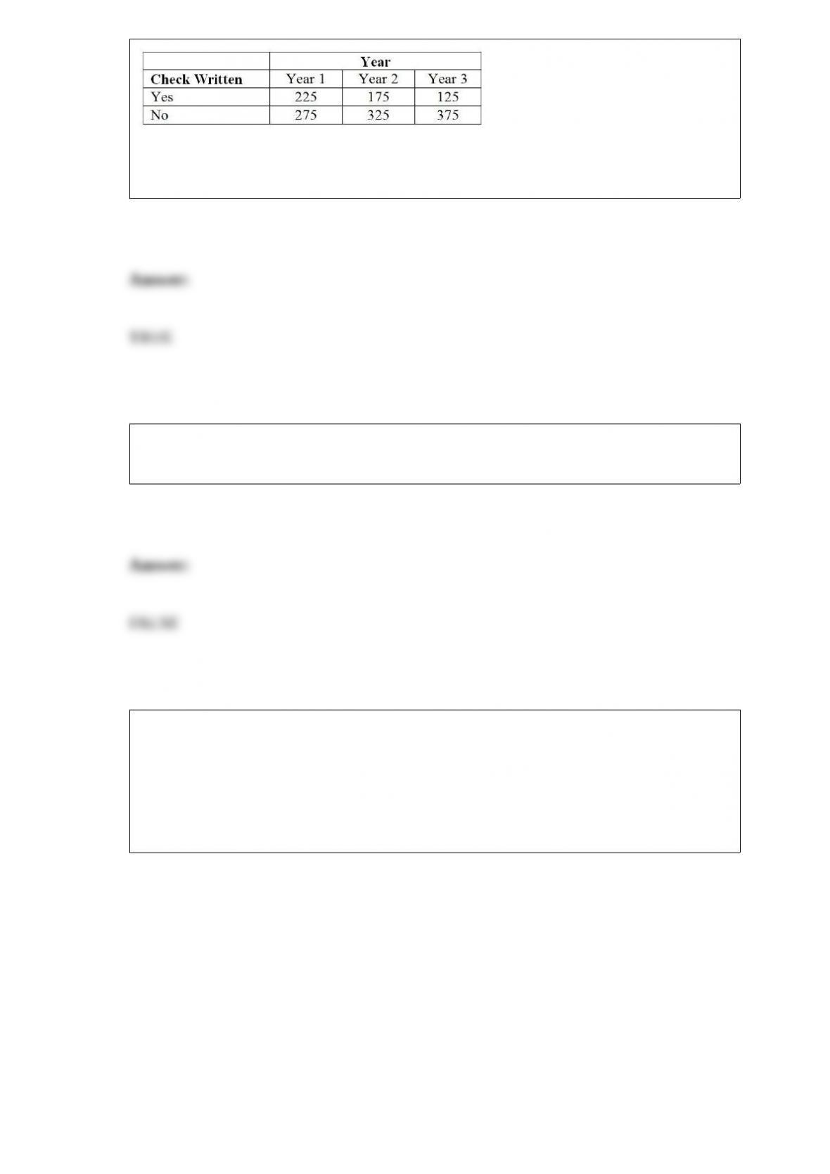
True or False: Referring to Table 12-6, there is sufficient evidence to conclude that the
proportions between year 1 and year 2 are different at a 0.05 level of significance.
True or False: The number of males selected in a sample of 5 students taken without
replacement from a class of 9 females and 18 males has a binomial distribution.
TABLE 17-1
A real estate builder wishes to determine how house size (House) is influenced by
family income (Income), family size (Size), and education of the head of household
(School). House size is measured in hundreds of square feet, income is measured in
thousands of dollars, and education is in years. The builder randomly selected 50
families and ran the multiple regression. Microsoft Excel output is provided below:
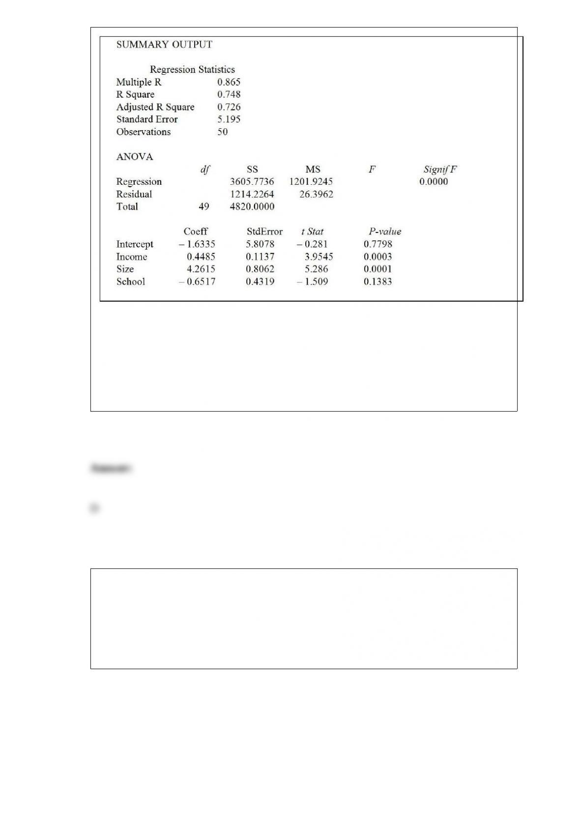
Referring to Table 17-1, what minimum annual income would an individual with a
family size of 4 and 16 years of education need to attain a predicted 10,000 square foot
home (House = 100)?
A) $44.14 thousand
B) $56.75 thousand
C) $178.33 thousand
D) $211.85 thousand
TABLE 10-2
A researcher randomly sampled 30 graduates of an MBA program and recorded data
concerning their starting salaries. Of primary interest to the researcher was the effect of
gender on starting salaries. The result of the pooled-variance t-test of the mean salaries
of the females (Population 1) and males (Population 2) in the sample is given below.
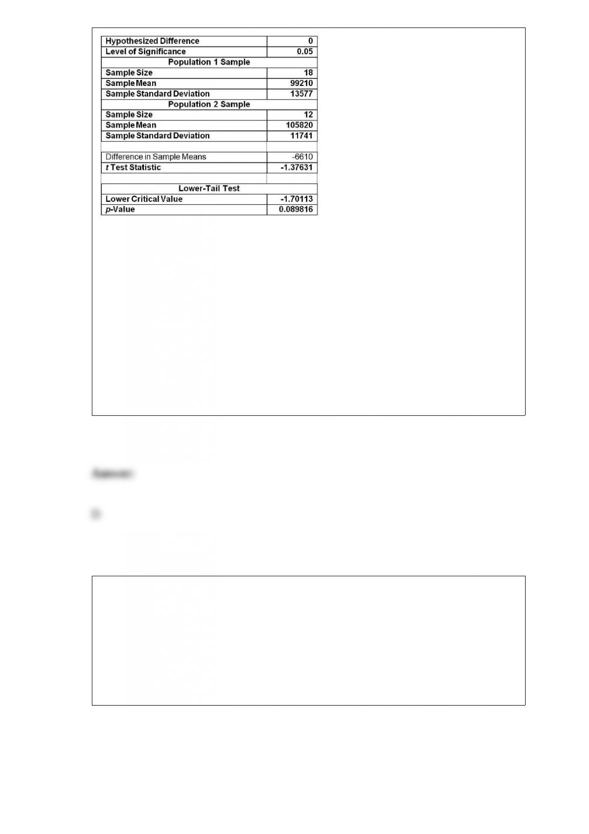
Referring to Table 10-2, the researcher was attempting to show statistically that the
female MBA graduates have a significantly lower mean starting salary than the male
MBA graduates. What assumptions were necessary to conduct this hypothesis test?
A) Both populations of salaries (male and female) must have approximate normal
distributions.
B) The population variances are approximately equal.
C) The samples were randomly and independently selected.
D) All of the above assumptions were necessary.
TABLE 17-2
One of the most common questions of prospective house buyers pertains to the cost of
heating in dollars (Y). To provide its customers with information on that matter, a large
real estate firm used the following 4 variables to predict heating costs: the daily
minimum outside temperature in degrees of Fahrenheit (X1), the amount of insulation in
inches (X2), the number of windows in the house (X3), and the age of the furnace in
years (X4). Given below are the EXCEL outputs of two regression models.
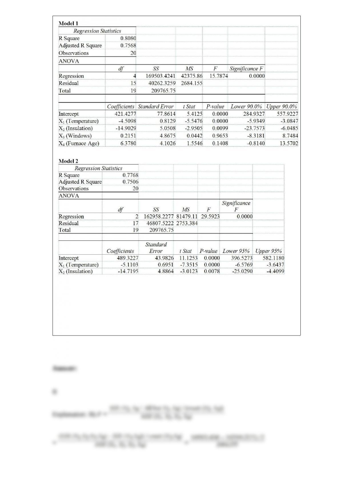
Referring to Table 17-2, what is the value of the partial F test statistic for H0 : β3 = β4 =
0 vs. H1 : At least one βj ≠0, j = 3, 4?
A) 0.820
B) 1.219
C) 1.382
D) 15.787
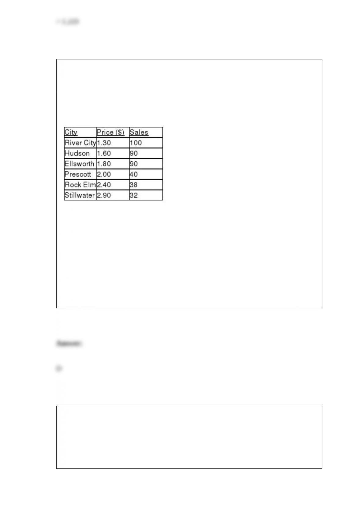
TABLE 13-2
A candy bar manufacturer is interested in trying to estimate how sales are influenced by
the price of their product. To do this, the company randomly chooses 6 small cities and
offers the candy bar at different prices. Using candy bar sales as the dependent variable,
the company will conduct a simple linear regression on the data below:
Referring to Table 13-2, what is the estimated slope for the candy bar price and sales
data?
A) 161.386
B) 0.784
C) -3.810
D) -48.193
TABLE 13-2
A candy bar manufacturer is interested in trying to estimate how sales are influenced by
the price of their product. To do this, the company randomly chooses 6 small cities and
offers the candy bar at different prices. Using candy bar sales as the dependent variable,
the company will conduct a simple linear regression on the data below:
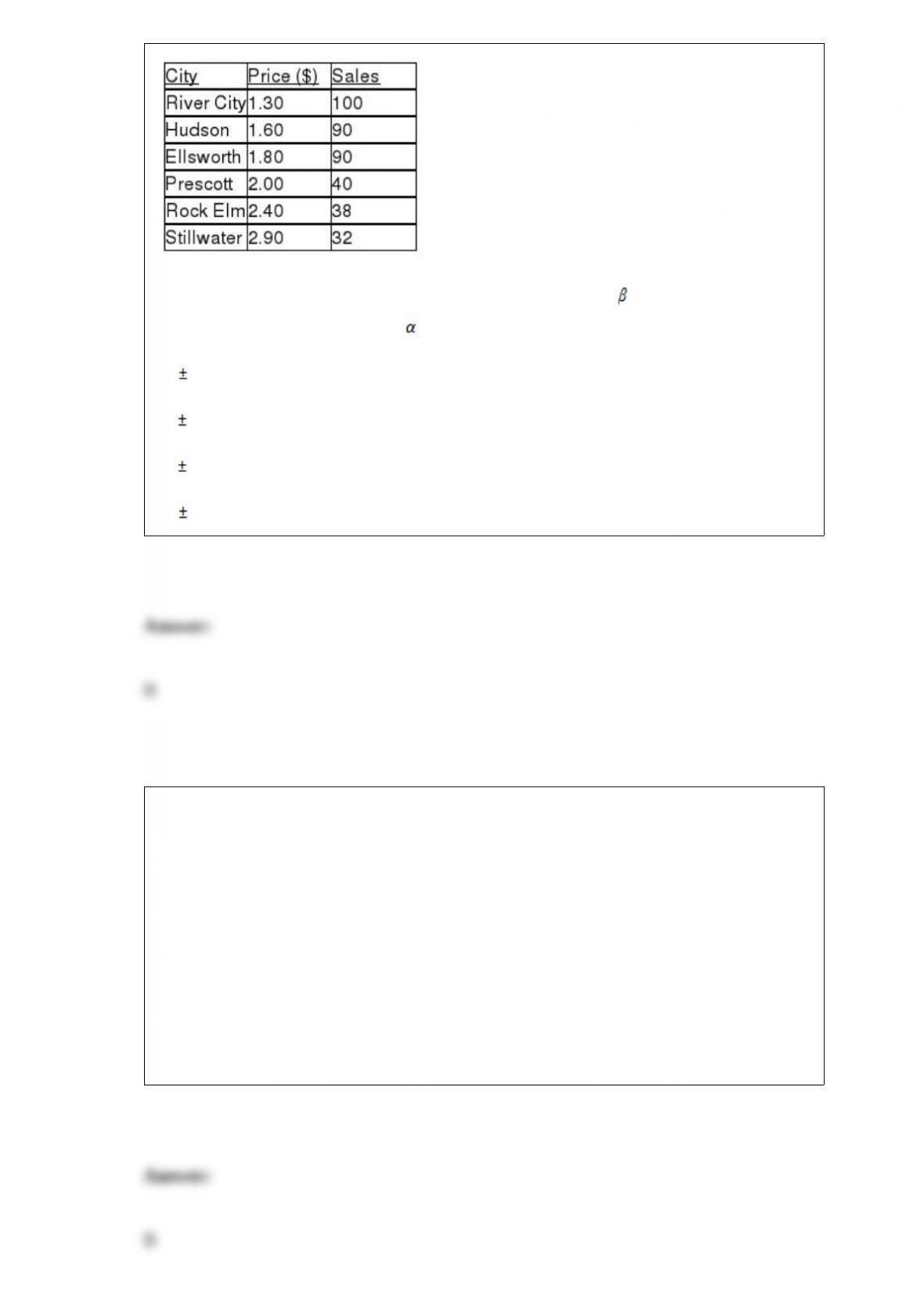
Referring to Table 13-2, to test that the regression coefficient, 1, is not equal to 0, what
would be the critical values? Use = 0.05.
A) 2.5706
B) 2.7764
C) 3.1634
D) 3.4954
Major league baseball salaries averaged $3.26 million with a standard deviation of $1.2
million in a recent year. Suppose a sample of 100 major league players was taken. Find
the approximate probability that the mean salary of the 100 players exceeded $3.5
million.
A) approximately 0
B) 0.0228
C) 0.9772
D) approximately 1

TABLE 1-1
The manager of the customer service division of a major consumer electronics company
is interested in determining whether the customers who have purchased a Blu-ray
player made by the company over the past 12 months are satisfied with their products.
Referring to Table 1-1, the possible responses to the question “How much time do you
use the Blu-ray player every week on the average?” result in
A) a nominal scale variable.
B) an ordinal scale variable.
C) an interval scale variable.
D) a ratio scale variable.
TABLE 15-3
A chemist employed by a pharmaceutical firm has developed a muscle relaxant. She
took a sample of 14 people suffering from extreme muscle constriction. She gave each a
vial containing a dose (X) of the drug and recorded the time to relief (Y) measured in
seconds for each. She fit a curvilinear model to this data. The results obtained by
Microsoft Excel follow
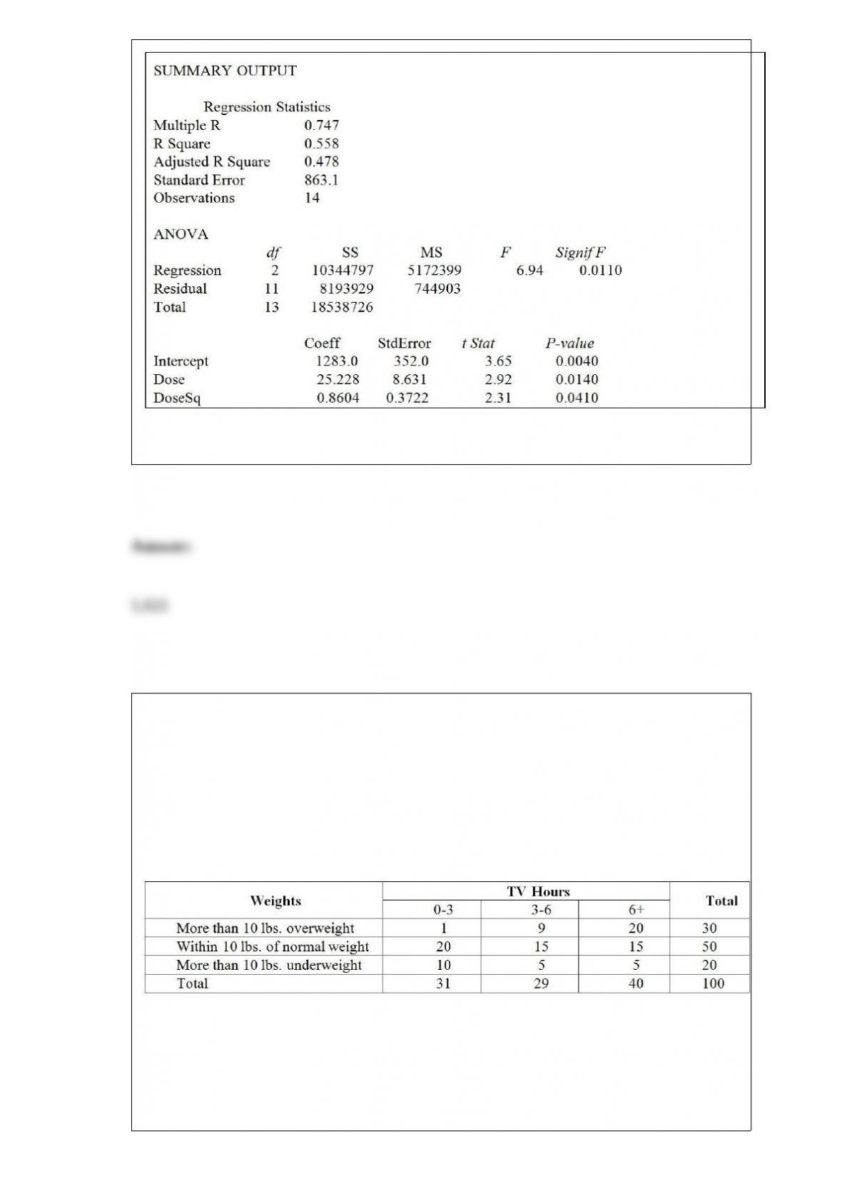
Referring to Table 15-3, the prediction of time to relief for a person receiving a dose of
10 units of the drug is ________.
TABLE 12-13
Recent studies have found that American children are more obese than in the past. The
amount of time children spent watching television has received much of the blame. A
survey of 100 ten-year-olds revealed the following with regards to weights and average
number of hours a day spent watching television. We are interested in testing whether
the mean number of hours spent watching TV and weights are independent at 1% level
of significance.
Referring to Table 12-13, if there is no connection between weights and average
number of hours spent watching TV, we should expect how many children to be
spending 3-6 hours on average watching TV and are more than 10 lbs. underweight?
A) 5
B) 5.8
C) 6.2
D) 8
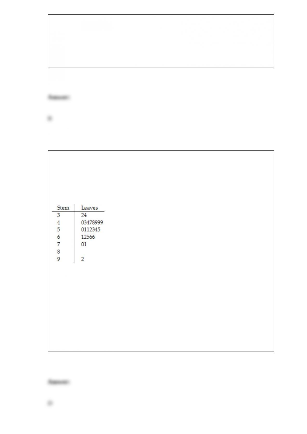
TABLE 2-4
A survey was conducted to determine how people rated the quality of programming
available on television. Respondents were asked to rate the overall quality from 0 (no
quality at all) to 100 (extremely good quality). The stem-and-leaf display of the data is
shown below.
Referring to Table 2-4, what percentage of the respondents rated overall television
quality with a rating from 50 through 75?
A) 11
B) 40
C) 44
D) 56
TABLE 9-8
One of the biggest issues facing e-retailers is the ability to turn browsers into buyers.
This is measured by the conversion rate, the percentage of browsers who buy something
in their visit to a site. The conversion rate for a company’s website was 10.1%. The
website at the company was redesigned in an attempt to increase its conversion rates. A
sample of 200 browsers at the redesigned site was selected. Suppose that 24 browsers
made a purchase. The company officials would like to know if there is evidence of an
increase in conversion rate at the 5% level of significance.
Referring to Table 9-8, the parameter the company officials are interested in is
A) the mean number of browsers who buy something in their visit to the company’s
website.
B) the total number of browsers who buy something in their visit to the company’s
website.
C) the mean number of company officials who buy something in their visit to the
company’s website.
D) the proportion of browsers who buy something in their visit to the company’s
website.
You have created a 95% confidence interval for with the result 10 15. What
decision will you make if you test H0: = 16 versus H1: ≠16 at = 0.05?
A) Reject H0 in favor of H1.
B) Do not reject H0 in favor of H1.
C) Fail to reject H0 in favor of H1.
D) We cannot tell what our decision will be from the information given.

TABLE 9-4
A drug company is considering marketing a new local anesthetic. The effective time of
the anesthetic the drug company is currently producing has a normal distribution with a
mean of 7.4 minutes with a standard deviation of 1.2 minutes. The chemistry of the new
anesthetic is such that the effective time should be normally distributed with the same
standard deviation, but the mean effective time may be lower. If it is lower, the drug
company will market the new anesthetic; otherwise, they will continue to produce the
older one. A sample size of 36 results in a sample mean of 7.1. A hypothesis test will be
done to help make the decision.
Referring to Table 9-4, the value of the test statistic is ________.
A second-order autoregressive model for average mortgage rate is:
Ratei = -2.0 + 1.8 (Rate)i-1 – 0.5 (Rate)i-2.
If the average mortgage rate in 2012 was 7.0, and in 2011 was 6.4, the forecast for 2013
is ________.
Suppose A and B are independent events where P(A) = 0.4 and P(B) = 0.5. Then P(A or
B) = ________.
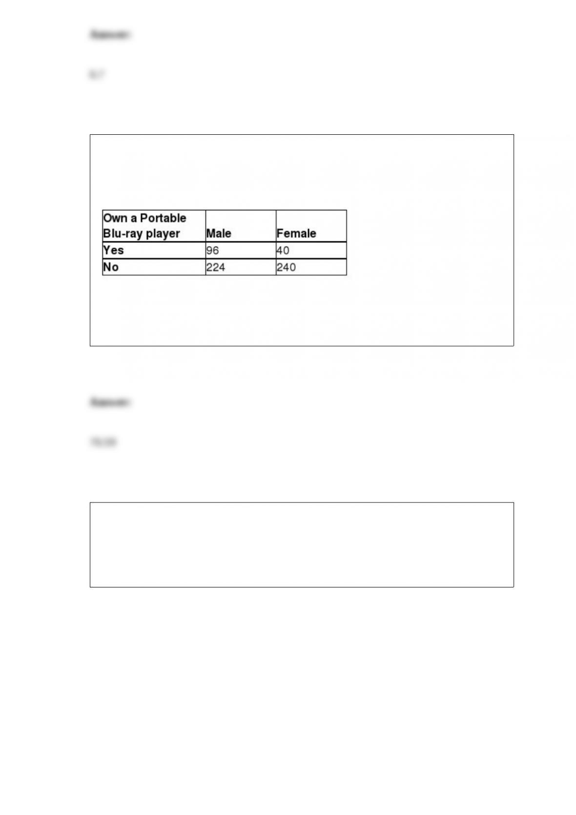
TABLE 2-14
The table below contains the number of people who own a portable Blu-ray player in a
sample of 600 broken down by gender.
Referring to Table 2-14, if the sample is a good representation of the population, we can
expect ________ percent of those who own a portable Blu-ray player in the population
will be males.
TABLE 13-5
The managing partner of an advertising agency believes that his company’s sales are
related to the industry sales. He uses Microsoft Excel to analyze the last 4 years of
quarterly data (i.e., n = 16) with the following results:
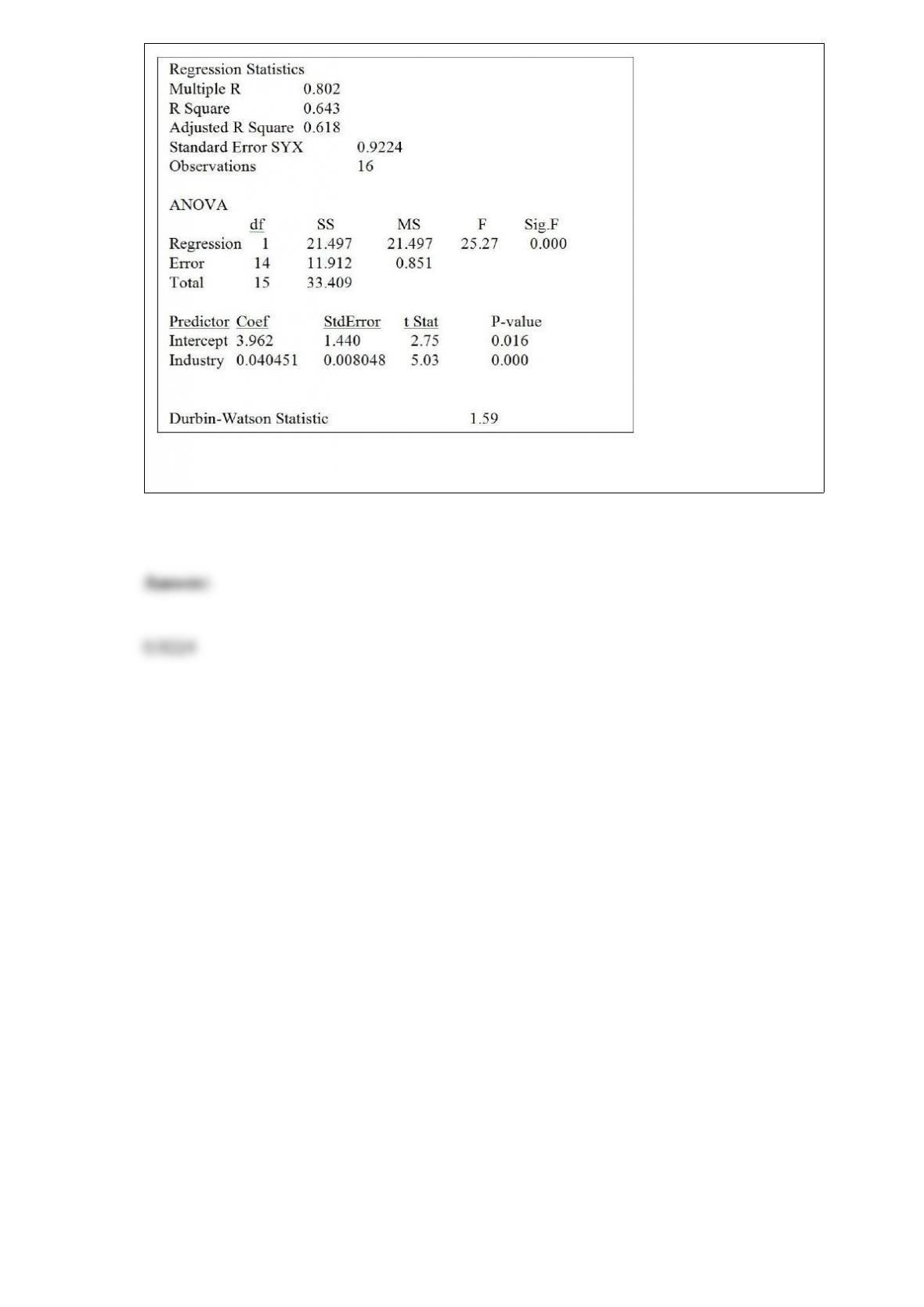
Referring to Table 13-5, the standard error of the estimate is ________.