True or False: Regression analysis is used for prediction, while correlation analysis is
used to measure the strength of the association between two numerical variables.
True or False: The sample proportion is an unbiased estimate of the population
proportion.
True or False: Coverage error can become an ethical issue if a particular group is
intentionally excluded from the frame.
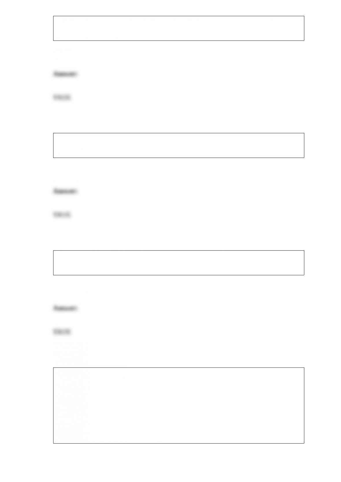
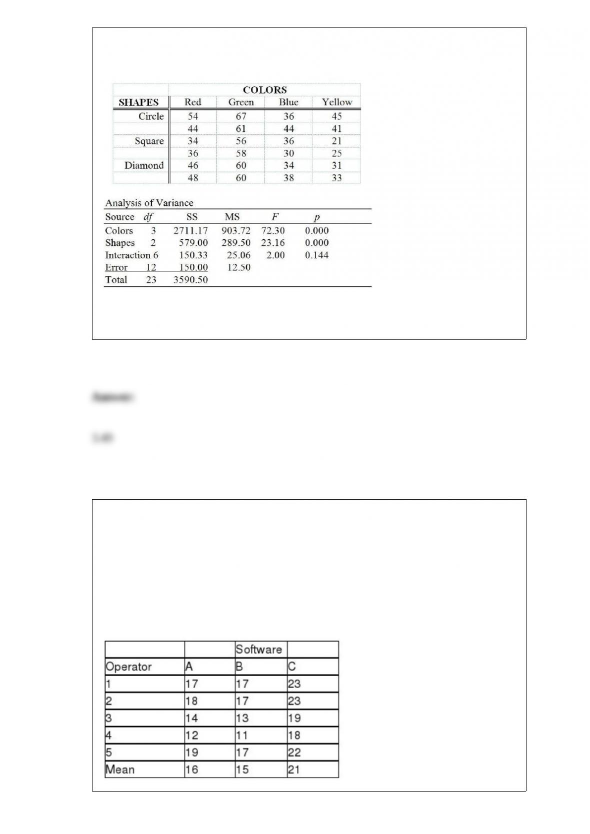
TABLE 11-8
An important factor in selecting database software is the time required for a user to
learn how to use the system. To evaluate three potential brands (A, B and C) of database
software, a company designed a test involving five different employees. To reduce
variability due to differences among employees, each of the five employees is trained
on each of the three different brands. The amount of time (in hours) needed to learn
each of the three different brands is given below:
Below is the Excel output for the randomized block design:
True or False: Referring to Table 11-8, the decision made at a 0.05 level of significance
on the F test for the block effects implies that the blocking has been advantageous in
reducing the experiment error.
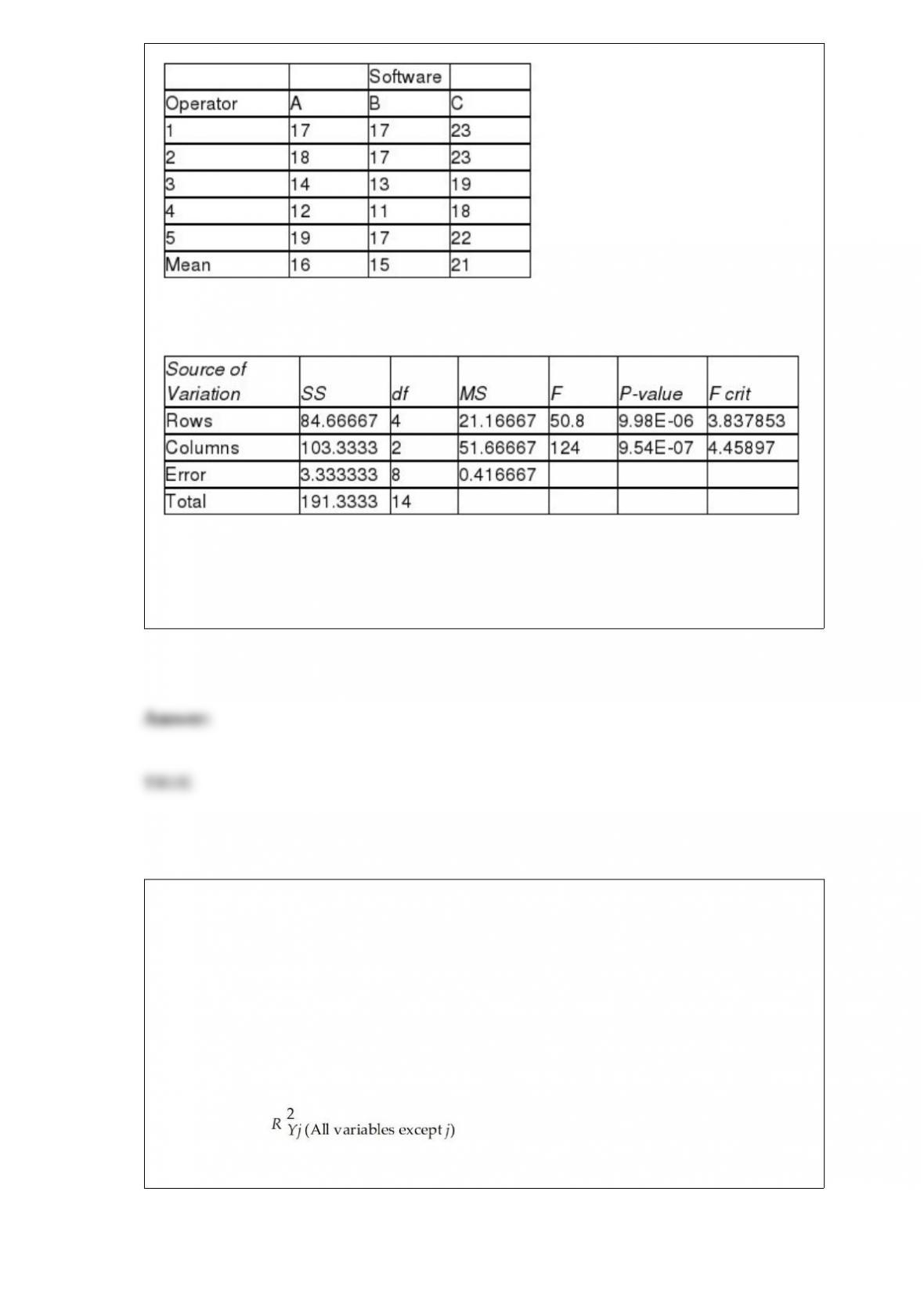
True or False: TABLE 17-10
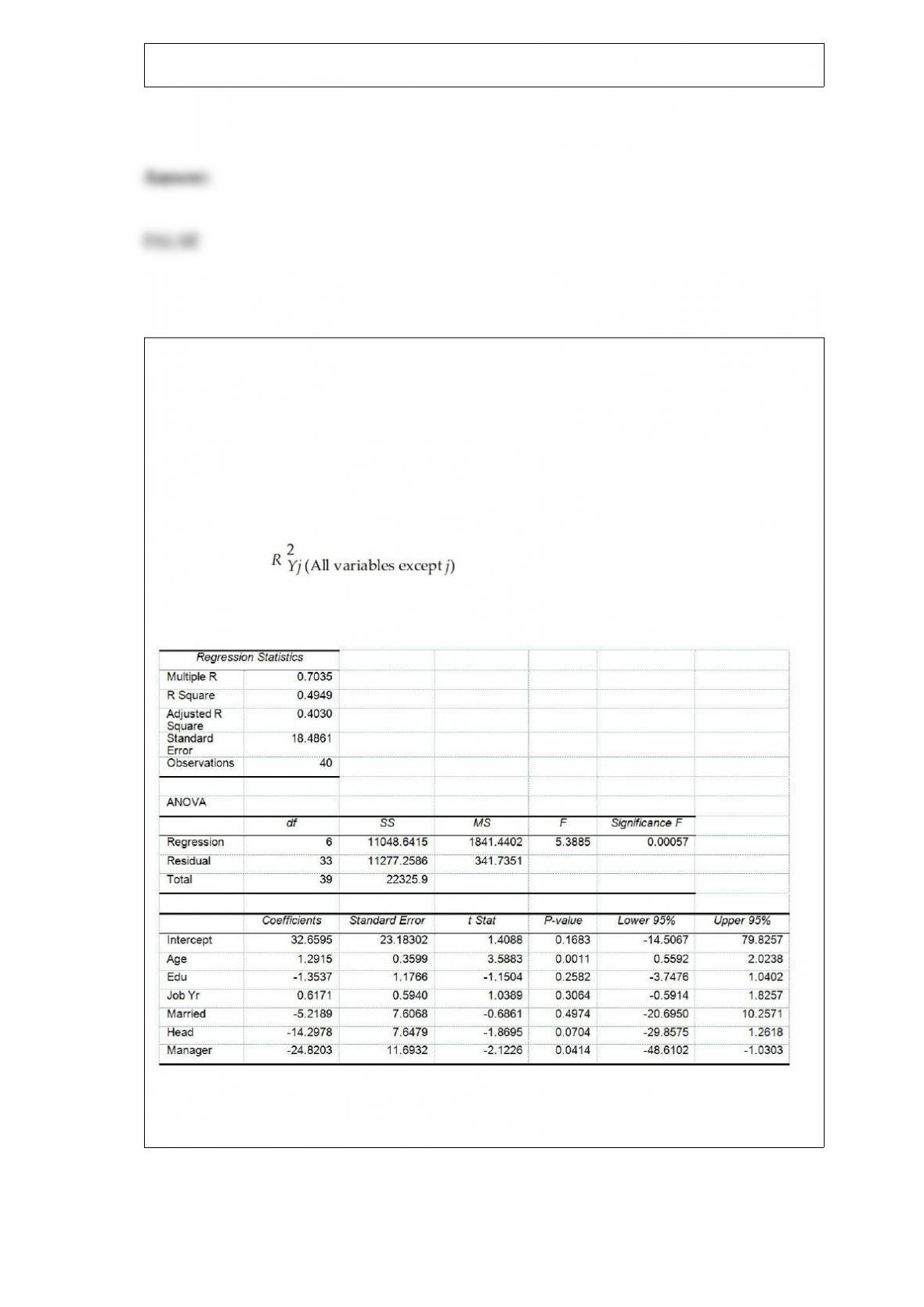
Given below are results from the regression analysis where the dependent variable is
the number of weeks a worker is unemployed due to a layoff (Unemploy) and the
independent variables are the age of the worker (Age), the number of years of education
received (Edu), the number of years at the previous job (Job Yr), a dummy variable for
marital status (Married: 1 = married, 0 = otherwise), a dummy variable for head of
household (Head: 1 = yes, 0 = no) and a dummy variable for management position
(Manager: 1 = yes, 0 = no). We shall call this Model 1. The coefficient of partial
determination ( ) of each of the 6 predictors are, respectively,
0.2807, 0.0386, 0.0317, 0.0141, 0.0958, and 0.1201.
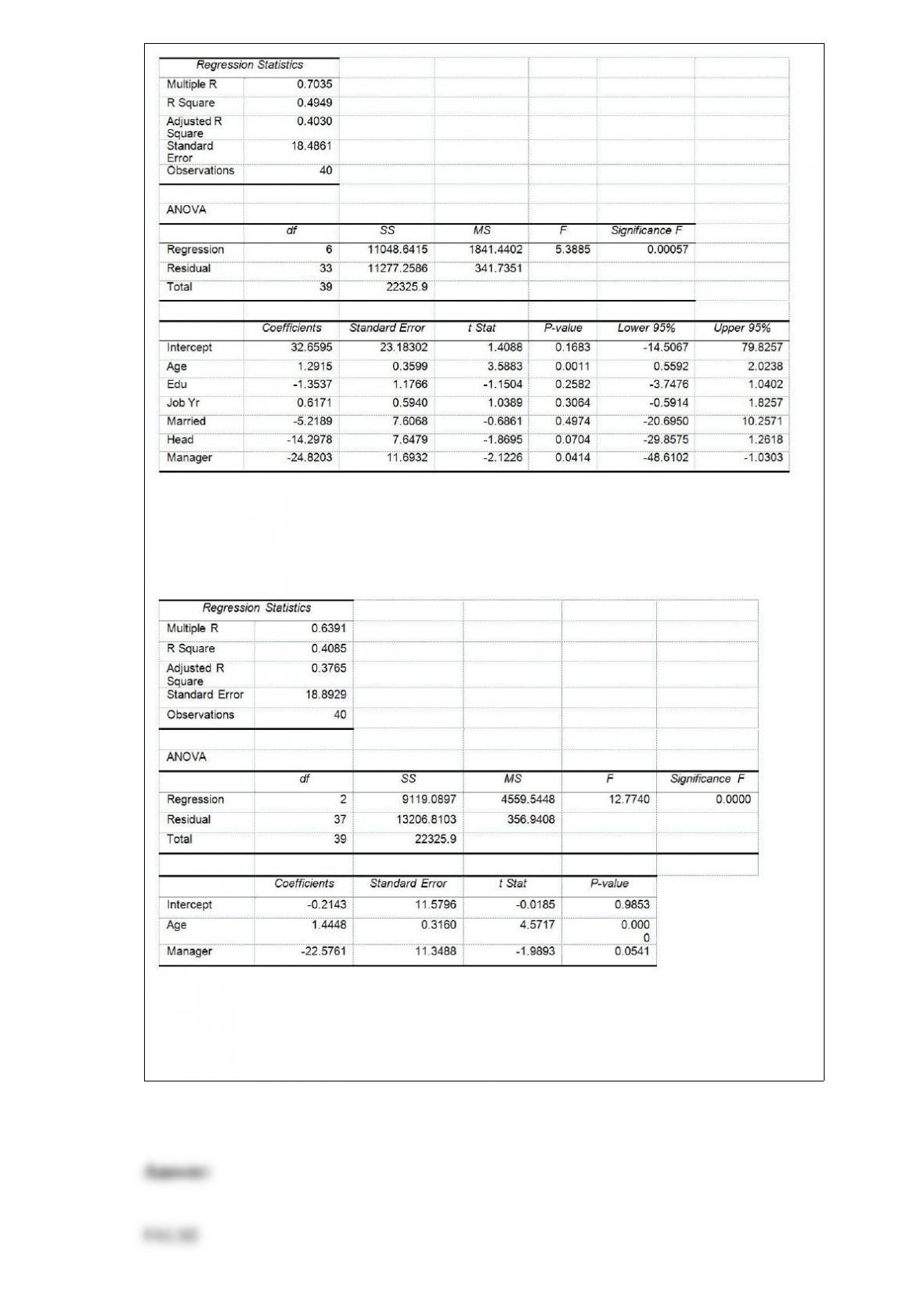
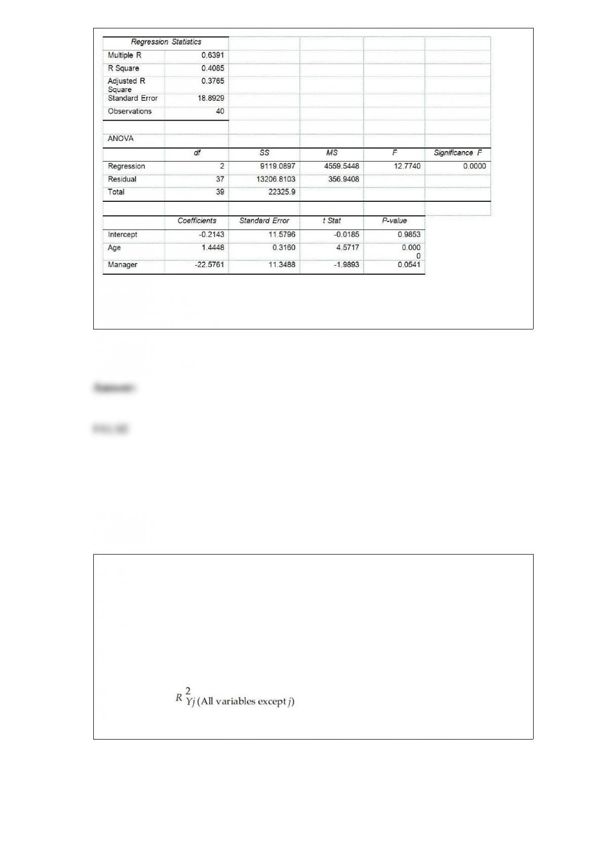
Model 2 is the regression analysis where the dependent variable is Unemploy and the
independent variables are Age and Manager. The results of the regression analysis are
given below:
Referring to Table 17-10, Model 1, the alternative hypothesis H1 : At least one of βj â
‰ 0 for j = 1, 2, 3, 4, 5, 6 implies that the number of weeks a worker is unemployed
due to a layoff is related to all of the explanatory variables.
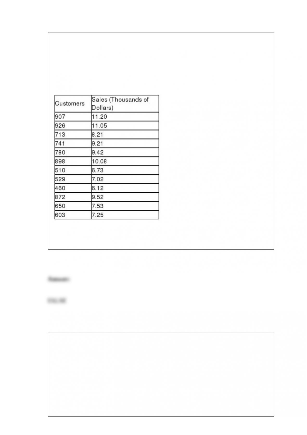
TABLE 13-10
The management of a chain electronic store would like to develop a model for
predicting the weekly sales (in thousands of dollars) for individual stores based on the
number of customers who made purchases. A random sample of 12 stores yields the
following results:
True or False: Referring to Table 13-10, 93.98% of the total variation in weekly sales
can be explained by the variation in the number of customers who make purchases.
TABLE 12-2
The dean of a college is interested in the proportion of graduates from his college who
have a job offer on graduation day. He is particularly interested in seeing if there is a
difference in this proportion for accounting and economics majors. In a random sample
of 100 of each type of major at graduation, he found that 65 accounting majors and 52
economics majors had job offers. If the accounting majors are designated as “Group 1”
and the economics majors are designated as “Group 2,” perform the appropriate
hypothesis test using a level of significance of 0.05.
True or False: Referring to Table 12-2, the null hypothesis should be rejected.
True or False: TABLE 17-10
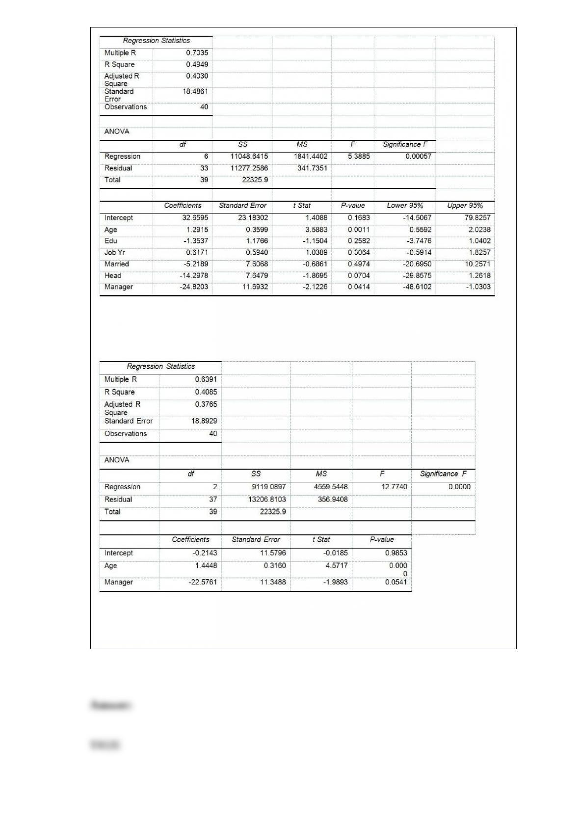
Given below are results from the regression analysis where the dependent variable is
the number of weeks a worker is unemployed due to a layoff (Unemploy) and the
independent variables are the age of the worker (Age), the number of years of education
received (Edu), the number of years at the previous job (Job Yr), a dummy variable for
marital status (Married: 1 = married, 0 = otherwise), a dummy variable for head of
household (Head: 1 = yes, 0 = no) and a dummy variable for management position
(Manager: 1 = yes, 0 = no). We shall call this Model 1. The coefficient of partial
determination ( ) of each of the 6 predictors are, respectively,
0.2807, 0.0386, 0.0317, 0.0141, 0.0958, and 0.1201.
Model 2 is the regression analysis where the dependent variable is Unemploy and the
independent variables are Age and Manager. The results of the regression analysis are
given below:
Referring to Table 17-10, Model 1, there is sufficient evidence that all of the
explanatory variables are related to the number of weeks a worker is unemployed due to
a layoff at a 10% level of significance.
True or False: TABLE 17-10
Given below are results from the regression analysis where the dependent variable is
the number of weeks a worker is unemployed due to a layoff (Unemploy) and the
independent variables are the age of the worker (Age), the number of years of education
received (Edu), the number of years at the previous job (Job Yr), a dummy variable for
marital status (Married: 1 = married, 0 = otherwise), a dummy variable for head of
household (Head: 1 = yes, 0 = no) and a dummy variable for management position
(Manager: 1 = yes, 0 = no). We shall call this Model 1. The coefficient of partial
determination ( ) of each of the 6 predictors are, respectively,
0.2807, 0.0386, 0.0317, 0.0141, 0.0958, and 0.1201.
Model 2 is the regression analysis where the dependent variable is Unemploy and the
independent variables are Age and Manager. The results of the regression analysis are
given below:
Referring to Table 17-10, Model 1, the null hypothesis H0 : β1 = β2= β3 = β4 = β5 = β6
= 0 implies that the number of weeks a worker is unemployed due to a layoff is not
affected by any of the explanatory variables.
True or False: TABLE 17-8
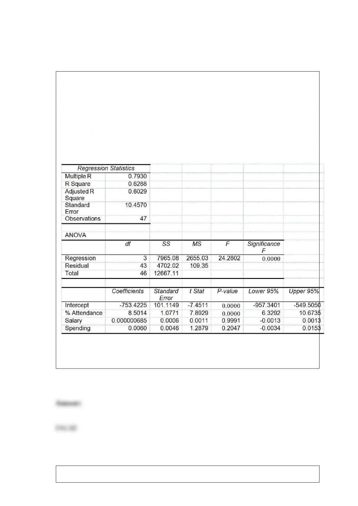
The superintendent of a school district wanted to predict the percentage of students
passing a sixth-grade proficiency test. She obtained the data on percentage of students
passing the proficiency test (% Passing), daily mean of the percentage of students
attending class (% Attendance), mean teacher salary in dollars (Salaries), and
instructional spending per pupil in dollars (Spending) of 47 schools in the state.
Following is the multiple regression output with Y = % Passing as the dependent
variable, X1 = % Attendance, X2 = Salaries and X3 = Spending:
Referring to Table 17-8, the null hypothesis H0 : β1 = β2 = β3 = 0 implies that the
percentage of students passing the proficiency test is not affected by some of the
explanatory variables.
True or False: Collinearity is present when there is a high degree of correlation between
independent variables.
True or False: The percentage distribution cannot be constructed from the frequency
distribution directly.
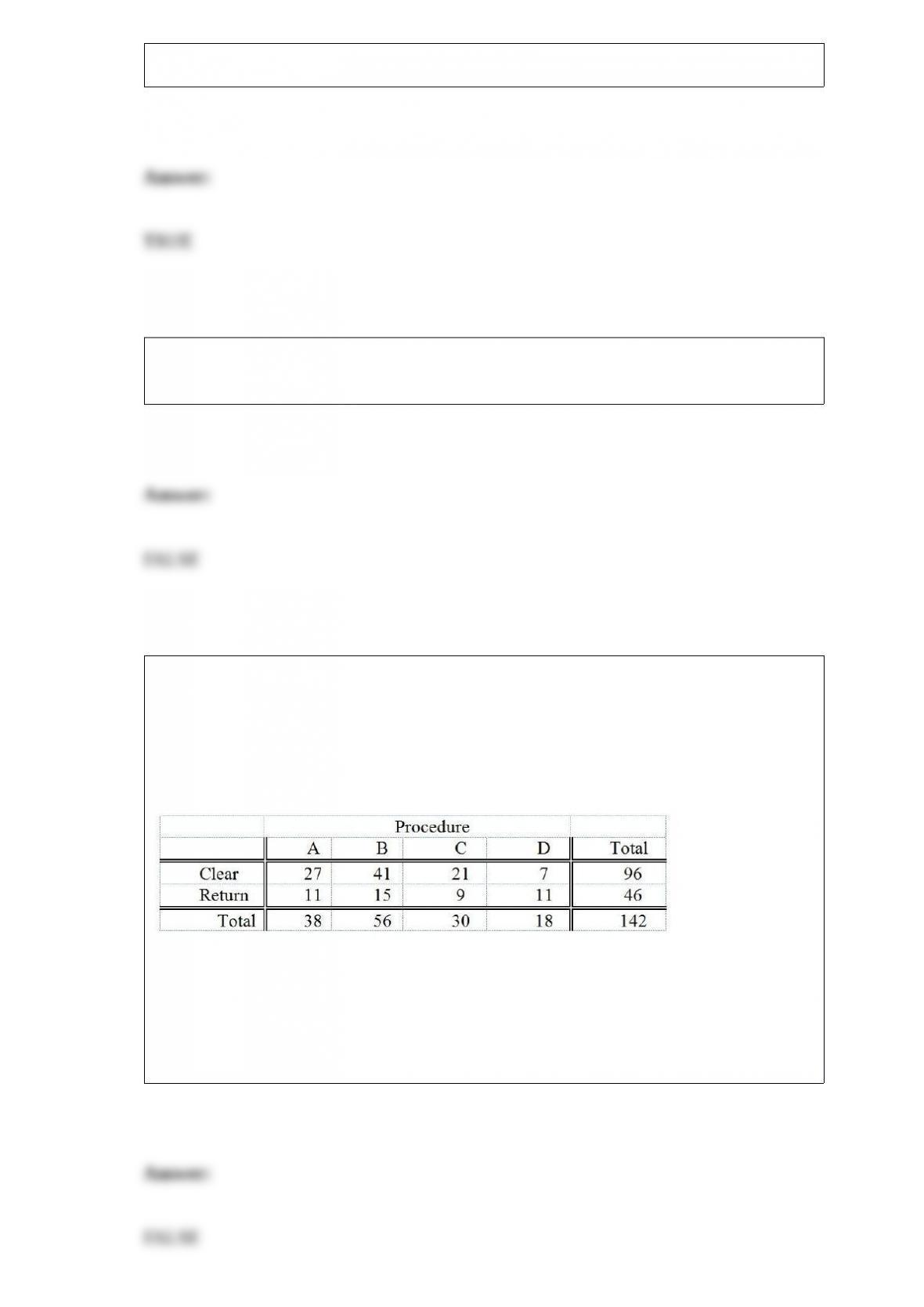
TABLE 12-5
Four surgical procedures currently are used to install pacemakers. If the patient does not
need to return for follow-up surgery, the operation is called a “clear” operation. A heart
center wants to compare the proportion of clear operations for the 4 procedures, and
collects the following numbers of patients from their own records:
They will use this information to test for a difference among the proportion of clear
operations using a chi-square test with a level of significance of 0.05.
True or False: Referring to Table 12-5, the decision made suggests that the 4 procedures
all have different proportions of clear operations.
True or False: The probability that a standard normal variable, Z, is below 1.96 is
0.4750.
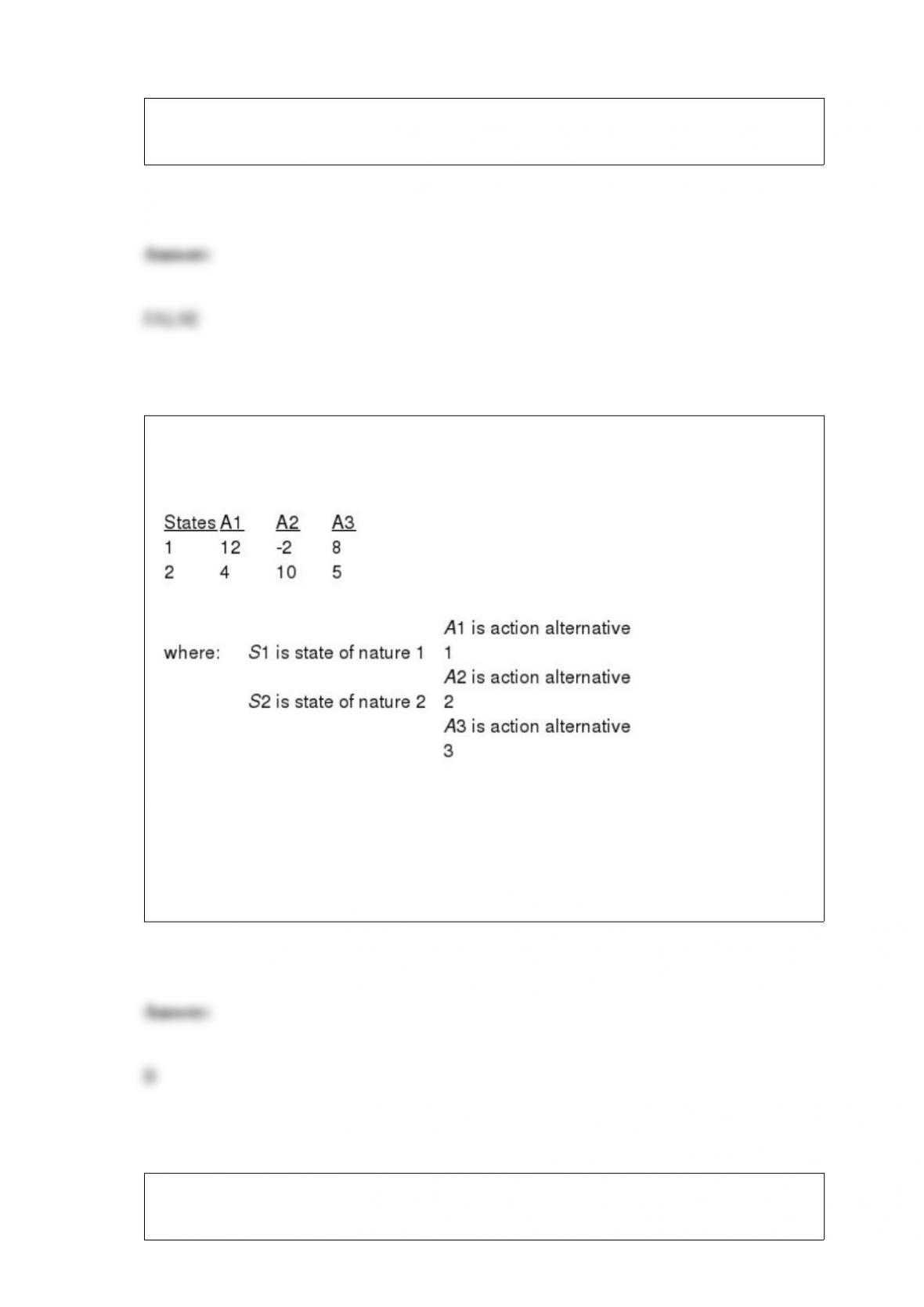
TABLE 19-1
The following payoff table shows profits associated with a set of 3 alternatives under 2
possible states of nature
Referring to Table 19-1, if the probability of S1 is 0.2 and S2 is 0.8, then the expected
monetary value of A1 is
A) 2.4.
B) 5.6.
C) 8.
D) 16.
The employees of a company were surveyed on questions regarding their educational
background (college degree or no college degree) and marital status (single or married).
Of the 600 employees, 400 had college degrees, 100 were single, and 60 were single
college graduates. The probability that an employee of the company is married and has
a college degree is
A) 0.0667.
B) 0.567.
C) 0.667.
D) 0.833.
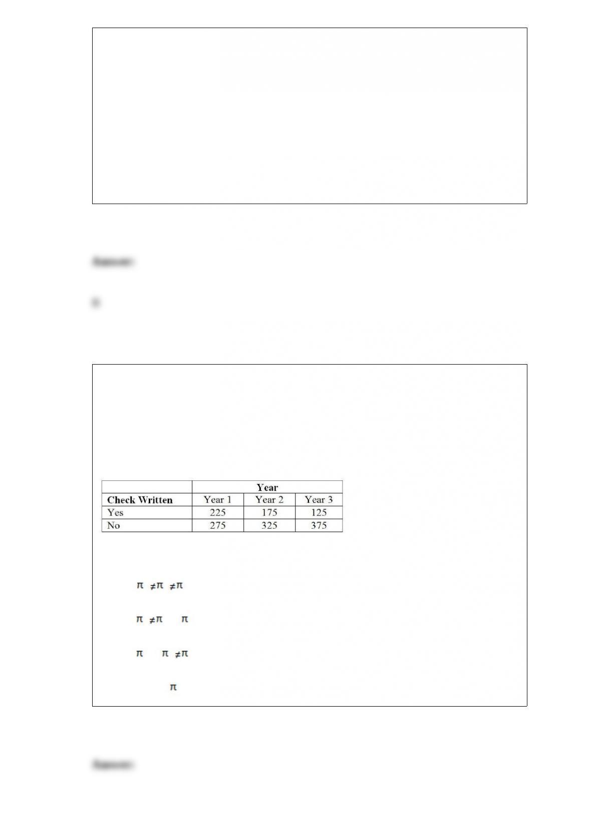
TABLE 12-6
According to an article in Marketing News, fewer checks are being written at the
grocery store checkout than in the past. To determine whether there is a difference in
the proportion of shoppers who pay by check among three consecutive years at a 0.05
level of significance, the results of a survey of 500 shoppers in three consecutive years
are obtained and presented below.
Referring to Table 12-6, what is the form of the alternative hypothesis?
A) H1 : 123
B) H1 : 1 2 = 3
C) H1 : 1 = 2 3
D) H1 : not all j are the same
In a one-way ANOVA, if the computed F statistic is greater than the critical F value you
may
A) reject H0 since there is evidence all the means differ.
B) reject H0 since there is evidence that not all the means are different.
C) not reject H0 since there is no evidence of a difference in the means.
D) not reject H0 because a mistake has been made.
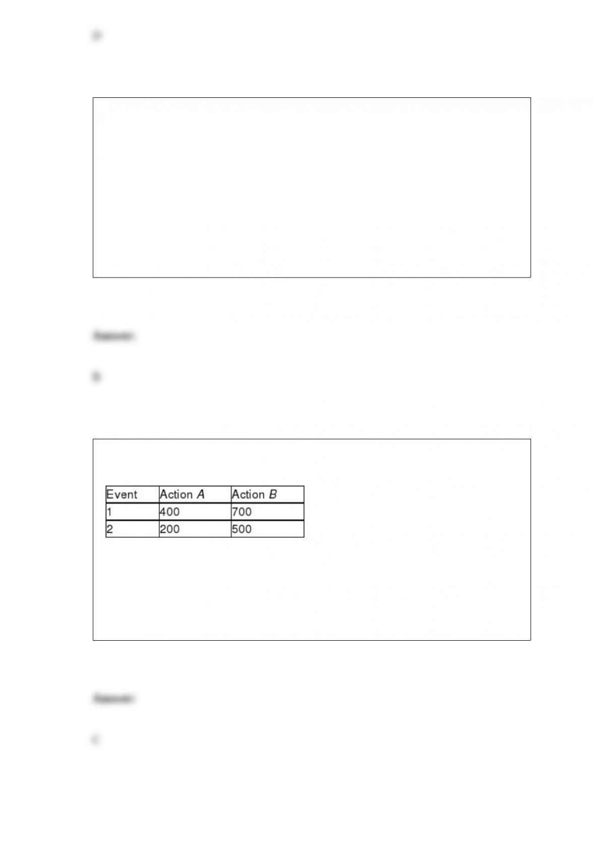
TABLE 19-2
The following payoff matrix is given in dollars.
Suppose the probability of Event 1 is 0.5 and Event 2 is 0.5.
Referring to Table 19-2, the return to risk ratio for Action B is
A) 0.167.
B) 3.0.
C) 6.0.
D) 9.0.
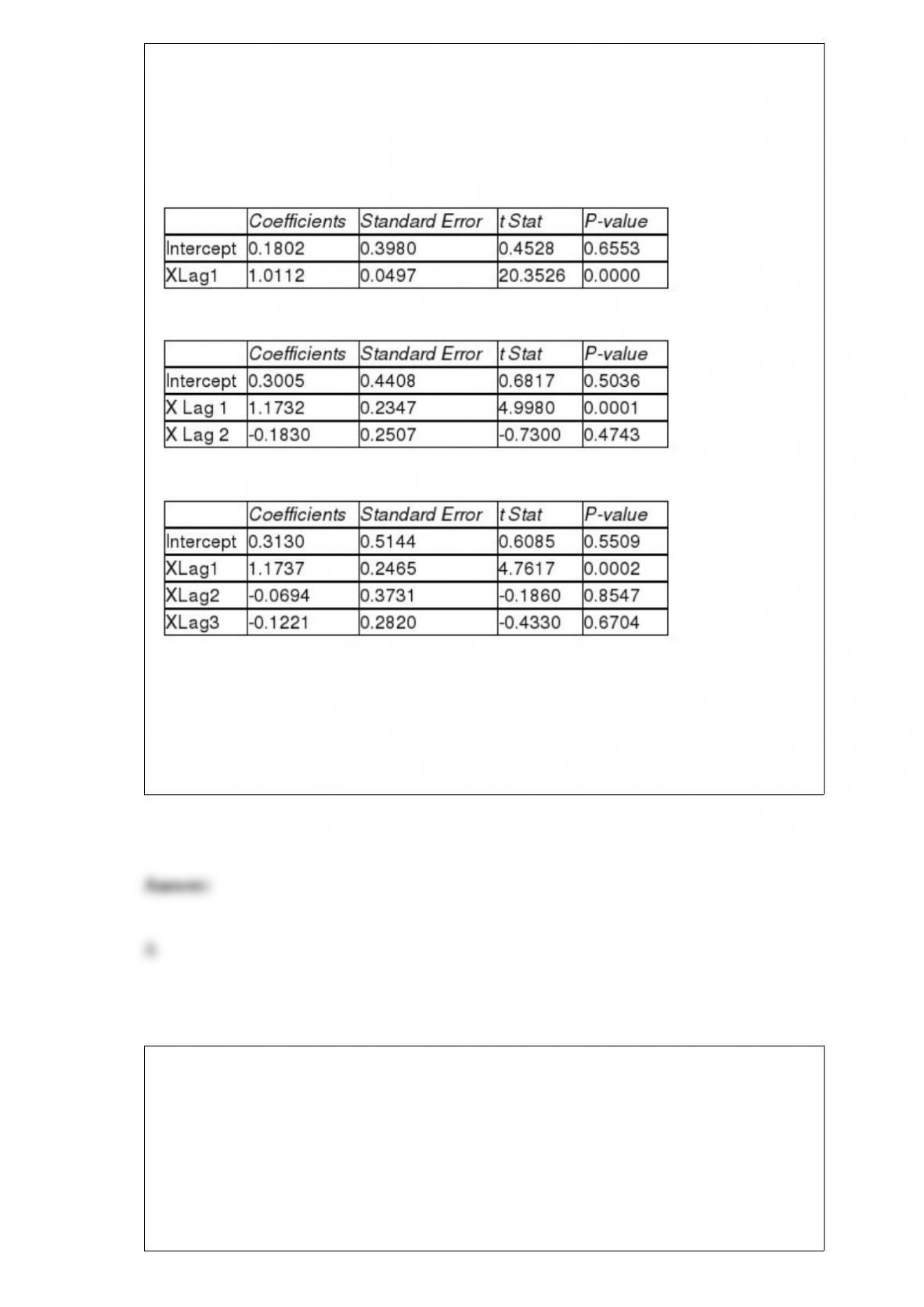
TABLE 16-9
Given below are EXCEL outputs for various estimated autoregressive models for a
company’s real operating revenues (in billions of dollars) from 1989 to 2012. From the
data, you also know that the real operating revenues for 2010, 2011, and 2012 are
11.7909, 11.7757 and 11.5537, respectively.
First-Order Autoregressive Model:
Second-Order Autoregressive Model:
Third-Order Autoregressive Model:
Referring to Table 16-9 and using a 5% level of significance, what is the appropriate
autoregressive model for the company’s real operating revenue?
A) First-Order Autoregressive Model
B) Second-Order Autoregressive Model
C) Third-Order Autoregressive Model
D) Any of the above.
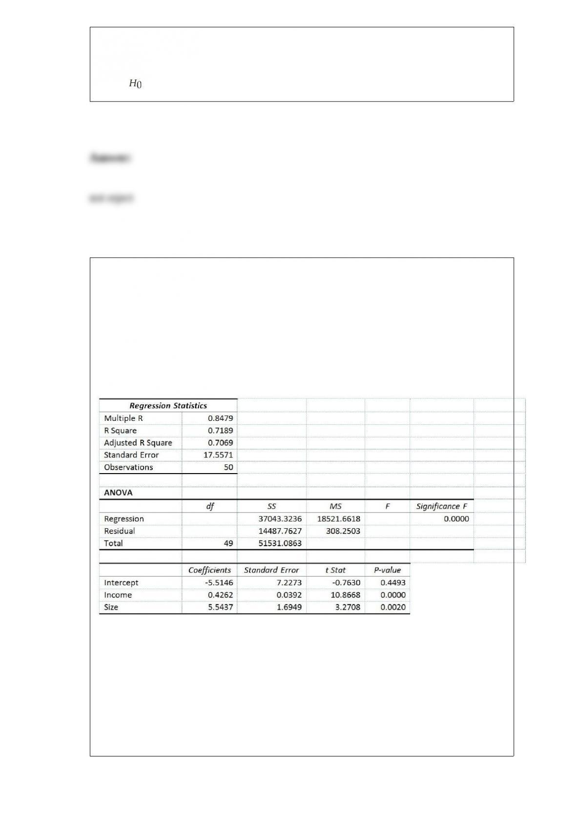
Referring to Table 14-4, at the 0.01 level of significance, what conclusion should the
builder draw regarding the inclusion of Size in the regression model?
TABLE 14-4
A real estate builder wishes to determine how house size (House) is influenced by
family income (Income) and family size (Size). House size is measured in hundreds of
square feet and income is measured in thousands of dollars. The builder randomly
selected 50 families and ran the multiple regression. Partial Microsoft Excel output is
provided below:
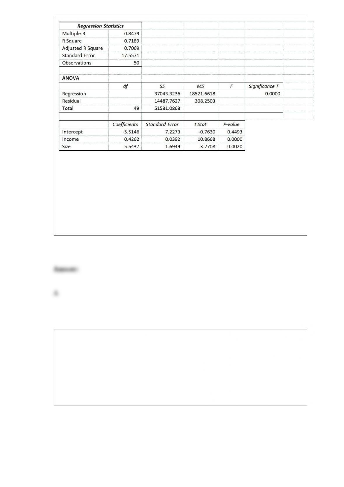
Also SSR (X1∣ X2) = 36400.6326 and SSR (X2∣ X1) = 3297.7917
A) Size is significant in explaining house size and should be included in the model
because its p-value is less than 0.01.
B) Size is significant in explaining house size and should be included in the model
because its p-value is more than 0.01.
C) Size is not significant in explaining house size and should not be included in the
model because its p-value is less than 0.01.
D) Size is not significant in explaining house size and should not be included in the
model because its p-value is more than 0.01.
TABLE 17-11
A logistic regression model was estimated in order to predict the probability that a
randomly chosen university or college would be a private university using information
on mean total Scholastic Aptitude Test score (SAT) at the university or college, the
room and board expense measured in thousands of dollars (Room/Brd), and whether the
TOEFL criterion is at least 550 (Toefl550 = 1 if yes, 0 otherwise.) The dependent
variable, Y, is school type (Type = 1 if private and 0 otherwise).
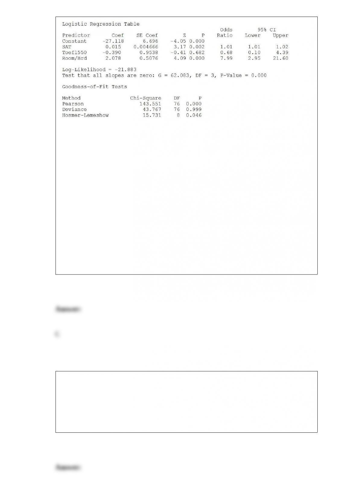
Referring to Table 17-11, which of the following is the correct interpretation for the
Tofel500 slope coefficient?
A) Holding constant the effect of the other variables, the estimated mean value of
school type is 0.39 lower when the school has a TOEFL criterion that is at least 550.
B) Holding constant the effect of the other variables, the estimated school type
decreases by 0.39 when the school has a TOEFL criterion that is at least 550.
C) Holding constant the effect of the other variables, the estimated natural logarithm of
the odds ratio of the school being a private school is 0.39 lower for a school that has a
TOEFL criterion that is at least 550 than one that does not.
D) Holding constant the effect of the other variables, the estimated probability of the
school being a private school is 0.39 lower for a school that has a TOEFL criterion that
is at least 550 than one that does not.
The risk seeker’s curve represents the utility of one who enjoys taking risks. Therefore,
the slope of the utility curve becomes ________ for large dollar amounts.
A) smaller
B) stable
C) larger
D) uncertain
In a multiple regression problem involving two independent variables, if b1 is computed
to be +2.0, it means that
A) the relationship between X1 and Y is significant.
B) the estimated mean of Y increases by 2 units for each increase of 1 unit of X1,
holding X2 constant.
C) the estimated mean of Y increases by 2 units for each increase of 1 unit of X1,
without regard to X2.
D) the estimated mean of Y is 2 when X1 equals zero.
Variation due to the inherent variability in a system of operation is called
A) special or assignable causes.
B) common or chance causes.
C) explained variation.
D) the standard deviation.
Which of the following sampling methods will more likely be susceptible to ethical
violation when used to form conclusions about the entire population?
A) simple random sample
B) cluster sample
C) judgment sample

D) stratified sample
Referring to Table 14-19, which of the following is the correct
interpretation for the Lawn Size slope coecient?
TABLE 14-19
The marketing manager for a nationally franchised lawn service
company would like to study the characteristics that differentiate
home owners who do and do not have a lawn service. A random
sample of 30 home owners located in a suburban area near a large
city was selected; 11 did not have a lawn service (code 0) and 19 had
a lawn service (code 1). Additional information available concerning
these 30 home owners includes family income (Income, in thousands
of dollars) and lawn size (Lawn Size, in thousands of square feet).
The PHStat output is given below:
A) Holding constant the effect of income, the estimated number of
lawn services purchased increases by 1.2804 for each increase of one
thousand square feet in lawn size.
B) Holding constant the effect of income, the estimated average
number of lawn services purchased increases by 1.2804 for each
increase of one thousand square feet in lawn size.
C) Holding constant the effect of income, the estimated probability of
purchasing a lawn service increases by 1.2804 for each increase of
one thousand square feet in lawn size.
D) Holding constant the effect of income, the estimated natural
logarithm of the odds ratio of purchasing a lawn service increases by
1.2804 for each increase of one thousand square feet in lawn size.
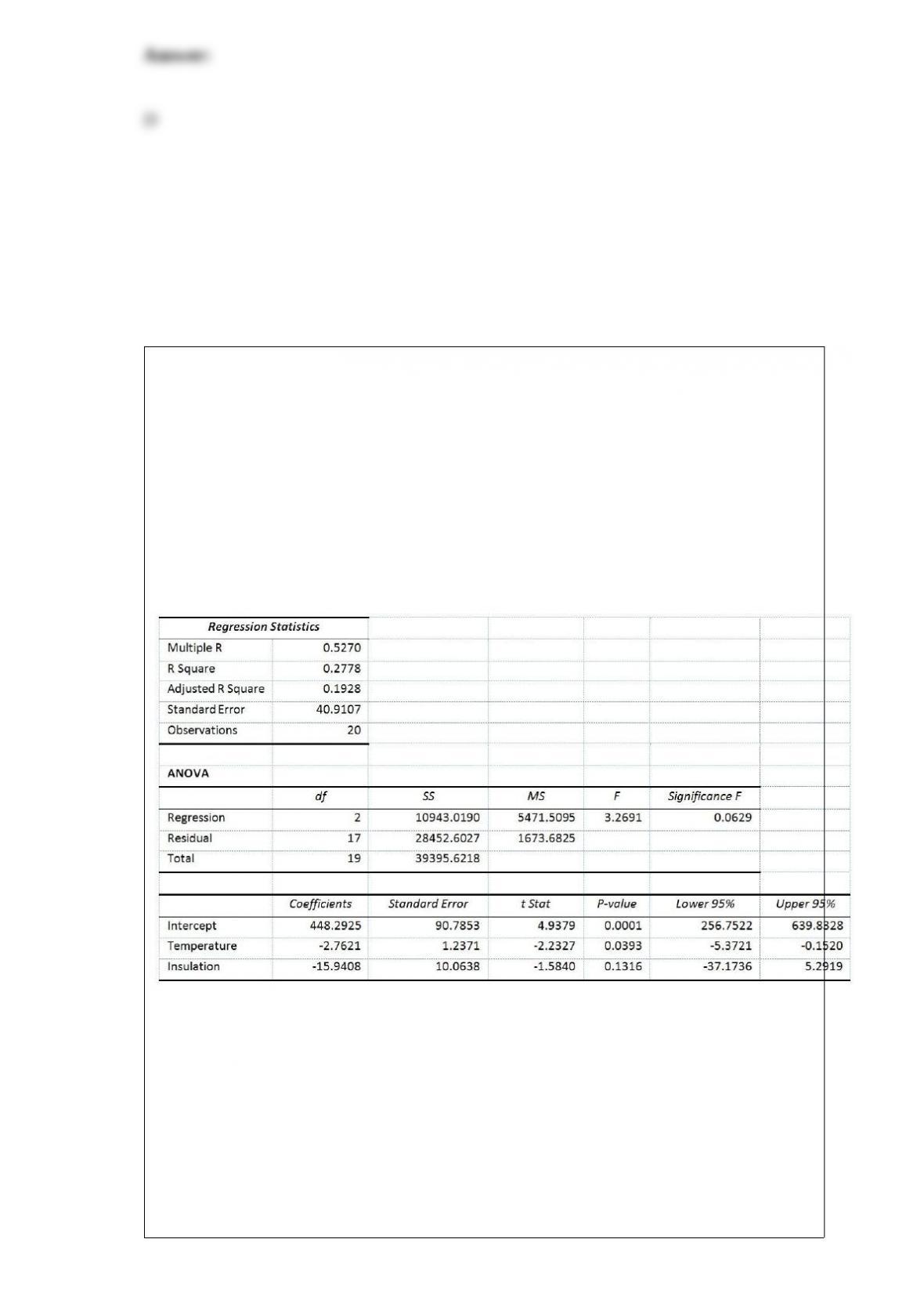
Referring to Table 14-6 and allowing for a 1% probability of committing a type I error,
what is the decision and conclusion for the test H0 : β1 = β2 = 0 vs. H1 : At least one βj
≠0, j = 1, 2?
TABLE 14-6
One of the most common questions of prospective house buyers pertains to the cost of
heating in dollars (Y). To provide its customers with information on that matter, a large
real estate firm used the following 2 variables to predict heating costs: the daily
minimum outside temperature in degrees of Fahrenheit (X1) and the amount of
insulation in inches (X2). Given below is EXCEL output of the regression model.
Also SSR (X1∣ X2) = 8343.3572 and SSR (X2∣ X1) = 4199.2672
A) Do not reject H0 and conclude that the 2 independent variables taken as a group
have significant linear effects on heating costs.
B) Do not reject H0 and conclude that the 2 independent variables taken as a group do
not have significant linear effects on heating costs.
C) Reject H0 and conclude that the 2 independent variables taken as a group have
significant linear effects on heating costs.
D) Reject H0 and conclude that the 2 independent variables taken as a group do not
have significant linear effects on heating costs.
True or False: The interquartile range is a measure of variation or dispersion in a set of
data.
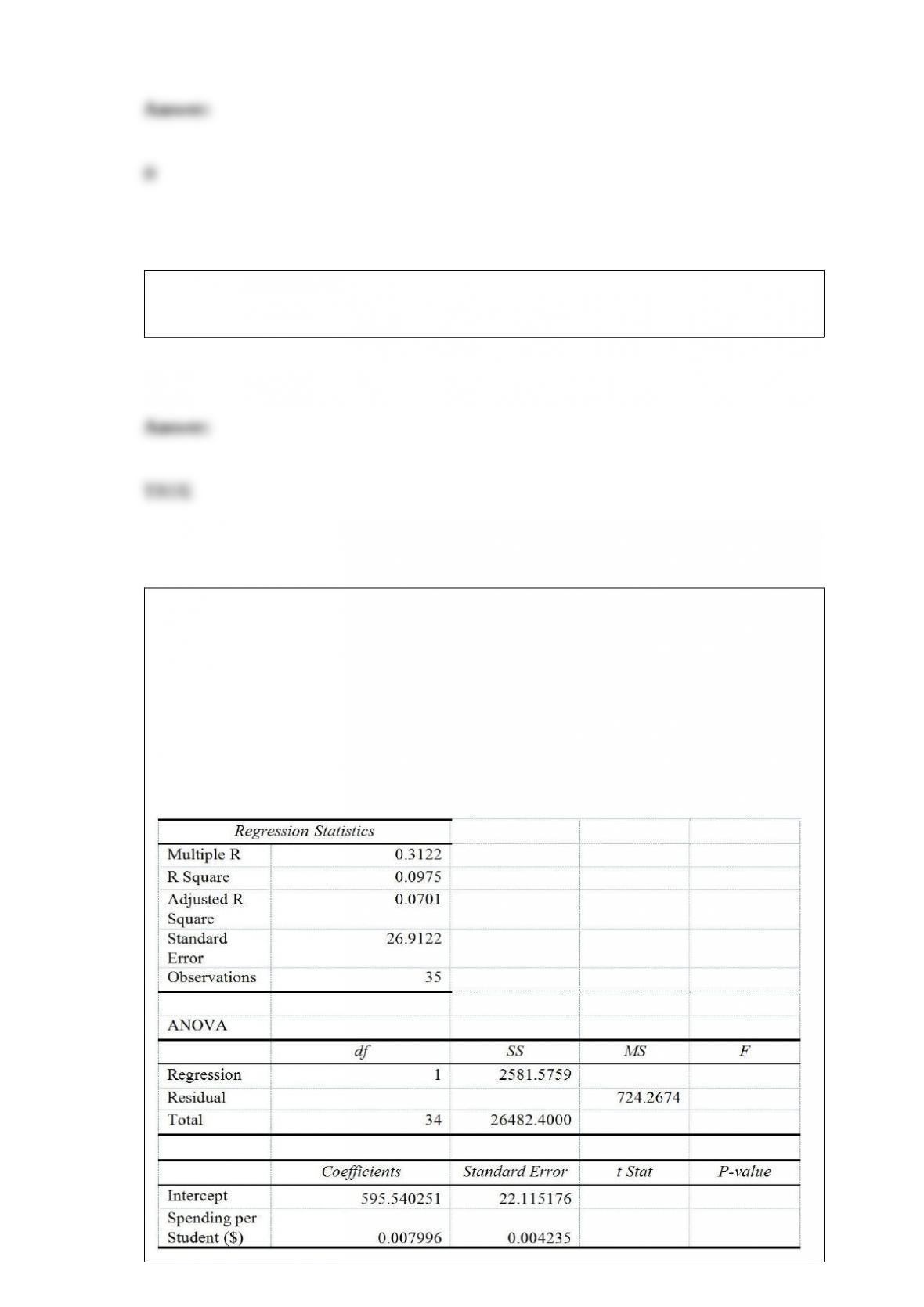
TABLE 13-13
In this era of tough economic conditions, voters increasingly ask the question: “Is the
educational achievement level of students dependent on the amount of money the state
in which they reside spends on education?” The partial computer output below is the
result of using spending per student ($) as the independent variable and composite score
which is the sum of the math, science and reading scores as the dependent variable on
35 states that participated in a study. The table includes only partial results.
Referring to Table 13-13, the decision on the test of whether spending per student
affects composite score using a 5% level of significance is to ________ (reject or not
reject) .
Referring to Table 14-4, at the 0.01 level of significance, what conclusion should the
builder reach regarding the inclusion of Income in the regression model?
TABLE 14-4
A real estate builder wishes to determine how house size (House) is influenced by
family income (Income) and family size (Size). House size is measured in hundreds of
square feet and income is measured in thousands of dollars. The builder randomly
selected 50 families and ran the multiple regression. Partial Microsoft Excel output is
provided below:
Also SSR (X1∣ X2) = 36400.6326 and SSR (X2∣ X1) = 3297.7917
A) Income is significant in explaining house size and should be included in the model
because its p-value is less than 0.01.
B) Income is significant in explaining house size and should be included in the model
because its p-value is more than 0.01.
C) Income is not significant in explaining house size and should not be included in the
model because its p-value is less than 0.01.
D) Income is not significant in explaining house size and should not be included in the
model because its p-value is more than 0.01.
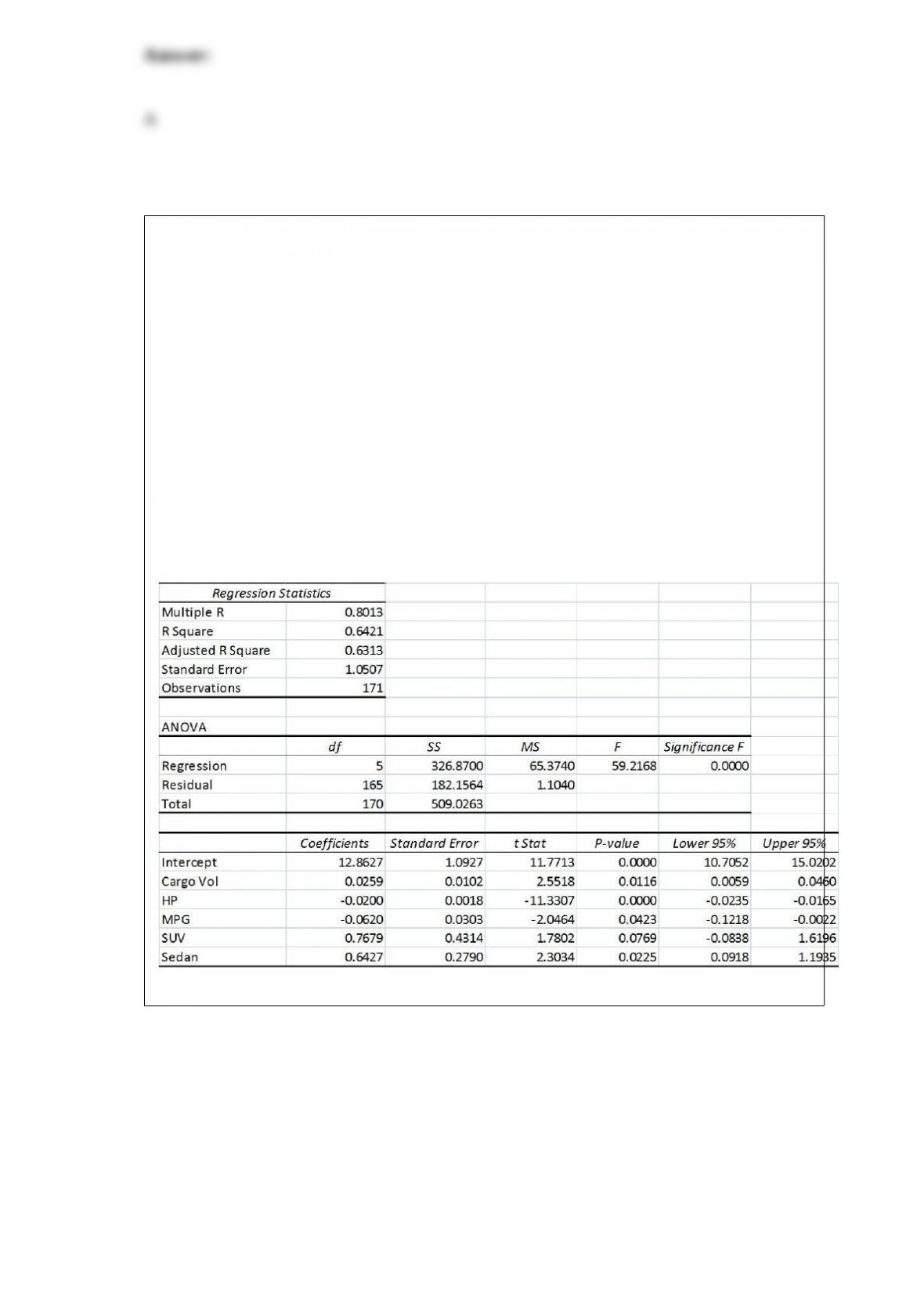
TABLE 17-9
What are the factors that determine the acceleration time (in sec.) from 0 to 60 miles per
hour of a car? Data on the following variables for 171 different vehicle models were
collected:
Accel Time: Acceleration time in sec.
Cargo Vol: Cargo volume in cu. ft.
HP: Horsepower
MPG: Miles per gallon
SUV: 1 if the vehicle model is an SUV with Coupe as the base when SUV and Sedan
are both 0
Sedan: 1 if the vehicle model is a sedan with Coupe as the base when SUV and Sedan
are both 0
The regression results using acceleration time as the dependent variable and the
remaining variables as the independent variables are presented below.
The various residual plots are as shown below.
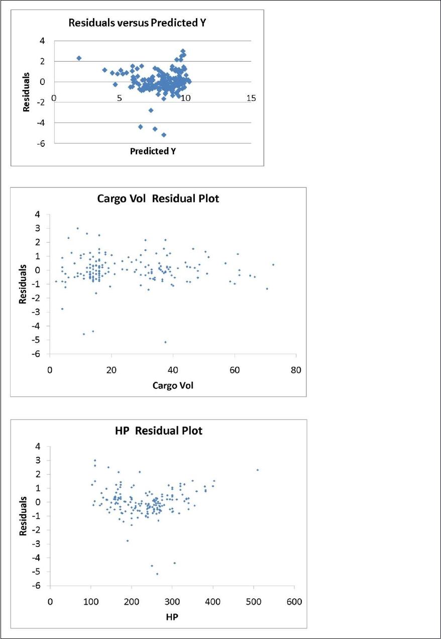
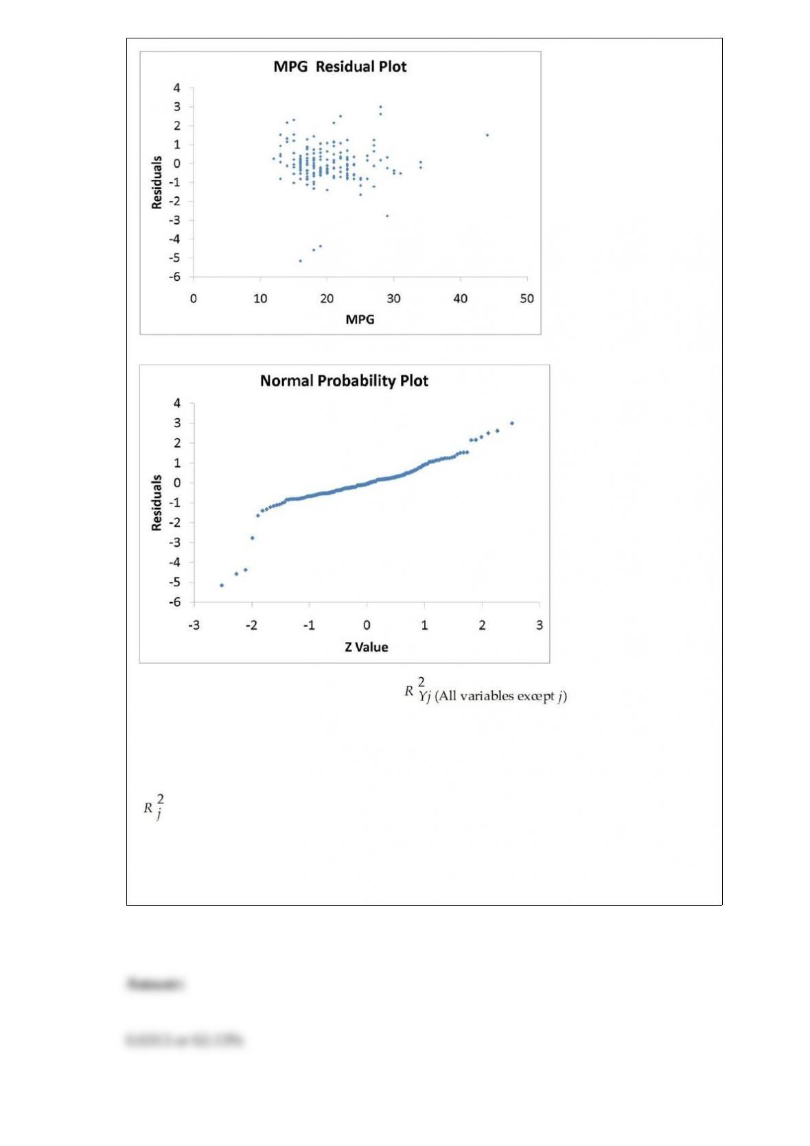
The coefficient of partial determination ( ) of each of the 5
predictors are, respectively, 0.0380, 0.4376, 0.0248, 0.0188, and 0.0312.
The coefficient of multiple determination for the regression model using each of the 5
variables Xj as the dependent variable and all other X variables as independent variables
( ) are, respectively, 0.7461, 0.5676, 0.6764, 0.8582, 0.6632.
Referring to Table 17-9, ________ of the variation in Accel Time can be explained by
the five independent variables after taking into consideration the number of independent
variables and the number of observations.

TABLE 9-12
A drug company is considering marketing a new local anesthetic. The effective time of
the anesthetic the drug company is currently producing has a normal distribution with a
mean of 7.4 minutes with a standard deviation of 1.2 minutes. The chemistry of the new
anesthetic is such that the effective time should be normally distributed with the same
standard deviation. The company will market the new local anesthetic as being better if
there is evidence that the population mean effective time is greater than the 7.4 minutes
of the current local anesthetic.
Referring to Table 9-12, if you select a sample of 25 new local anesthetics and are
willing to have a level of significance of 0.05, the probability of the company not
marketing the new local anesthetic when it is not better is ________.
A debate team of 4 is to be chosen from a class of 35. There are two twin brothers in the
class. How many possible ways can the team be formed which will include both of the
twin brothers?
TABLE 3-3
The ordered array below represents the number of vitamin supplements sold by a health
food store in a sample of 16 days.
19, 19, 20, 20, 22, 23, 25, 26, 27, 30, 33, 34, 35, 36, 38, 41
Note: For this sample, the sum of the values is 448, and the sum of the squared
differences between each value and the mean is 812.
Referring to Table 3-3, is the number of vitamin supplements sold in this sample right-
or left-skewed?
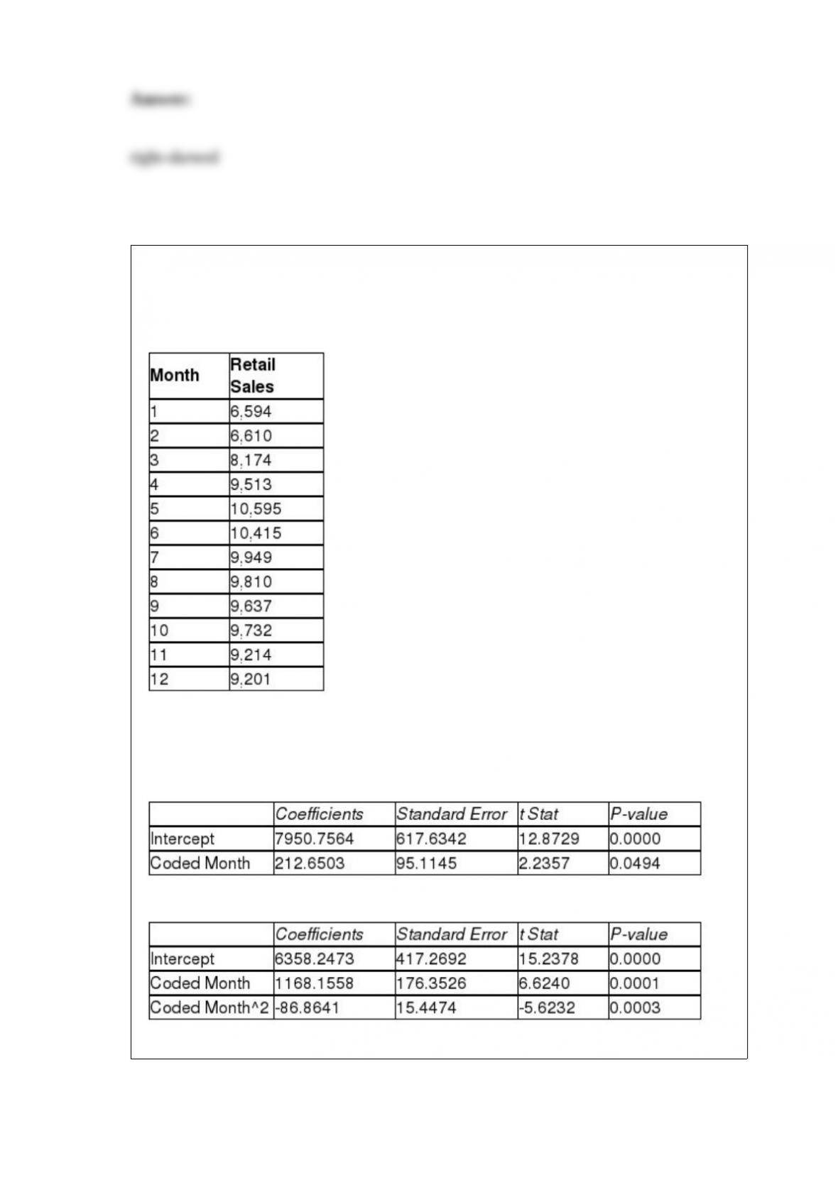
TABLE 16-13
Given below is the monthly time-series data for U.S. retail sales of building materials
over a specific year.
The results of the linear trend, quadratic trend, exponential trend, first-order
autoregressive, second-order autoregressive and third-order autoregressive model are
presented below in which the coded month for the 1st month is 0:
Linear trend model:
Quadratic trend model:
Exponential trend model:
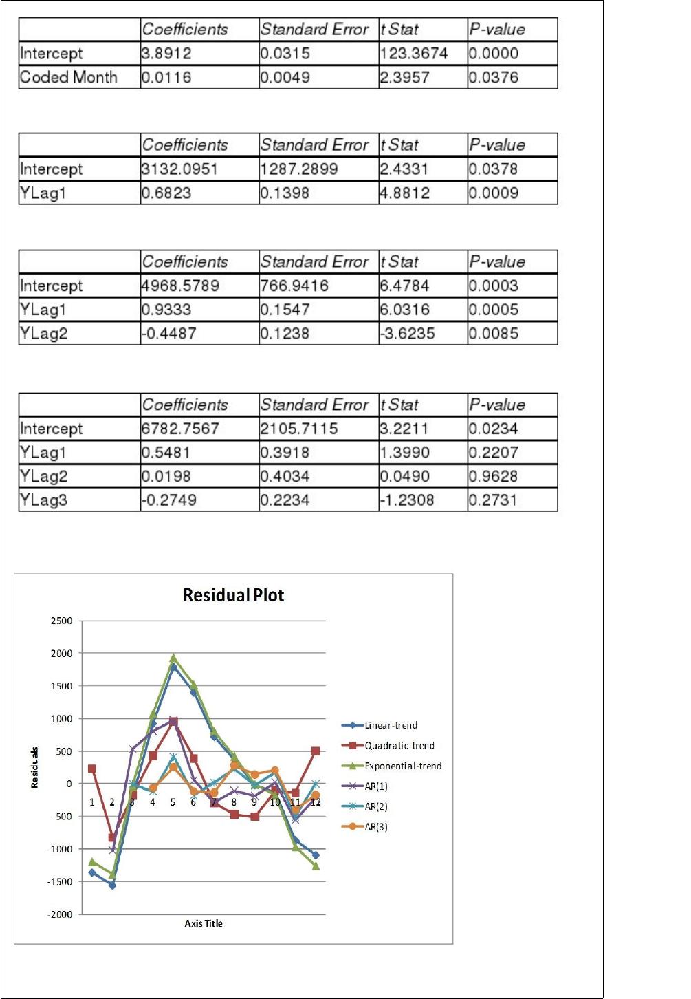
First-order autoregressive:
Second-order autoregressive:
Third-order autoregressive:
Below is the residual plot of the various models:
Referring to Table 16-13, what is the value of the t test statistic for testing the
appropriateness of the third-order autoregressive model?
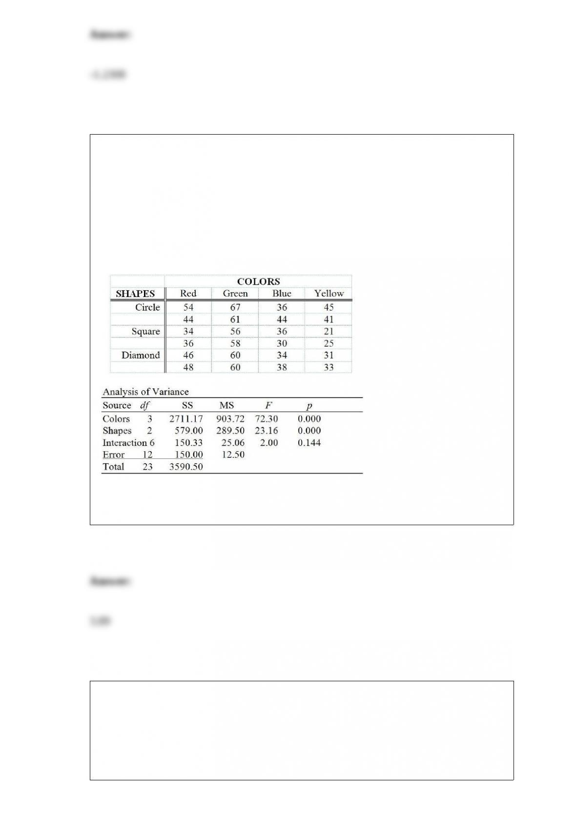
TABLE 11-9
The marketing manager of a company producing a new cereal aimed for children wants
to examine the effect of the color and shape of the box’s logo on the approval rating of
the cereal. He combined 4 colors and 3 shapes to produce a total of 12 designs. Each
logo was presented to 2 different groups (a total of 24 groups) and the approval rating
for each was recorded and is shown below. The manager analyzed these data using the
α = 0.05 level of significance for all inferences.
Referring to Table 11-9, the critical value in the test for significant differences between
shapes is ________.
TABLE 11-9
The marketing manager of a company producing a new cereal aimed for children wants
to examine the effect of the color and shape of the box’s logo on the approval rating of
the cereal. He combined 4 colors and 3 shapes to produce a total of 12 designs. Each
logo was presented to 2 different groups (a total of 24 groups) and the approval rating
for each was recorded and is shown below. The manager analyzed these data using the
α = 0.05 level of significance for all inferences.
Referring to Table 11-9, the critical value of the test for significant differences between
colors is ________.
TABLE 11-8
An important factor in selecting database software is the time required for a user to
learn how to use the system. To evaluate three potential brands (A, B and C) of database
software, a company designed a test involving five different employees. To reduce
variability due to differences among employees, each of the five employees is trained
on each of the three different brands. The amount of time (in hours) needed to learn
each of the three different brands is given below:
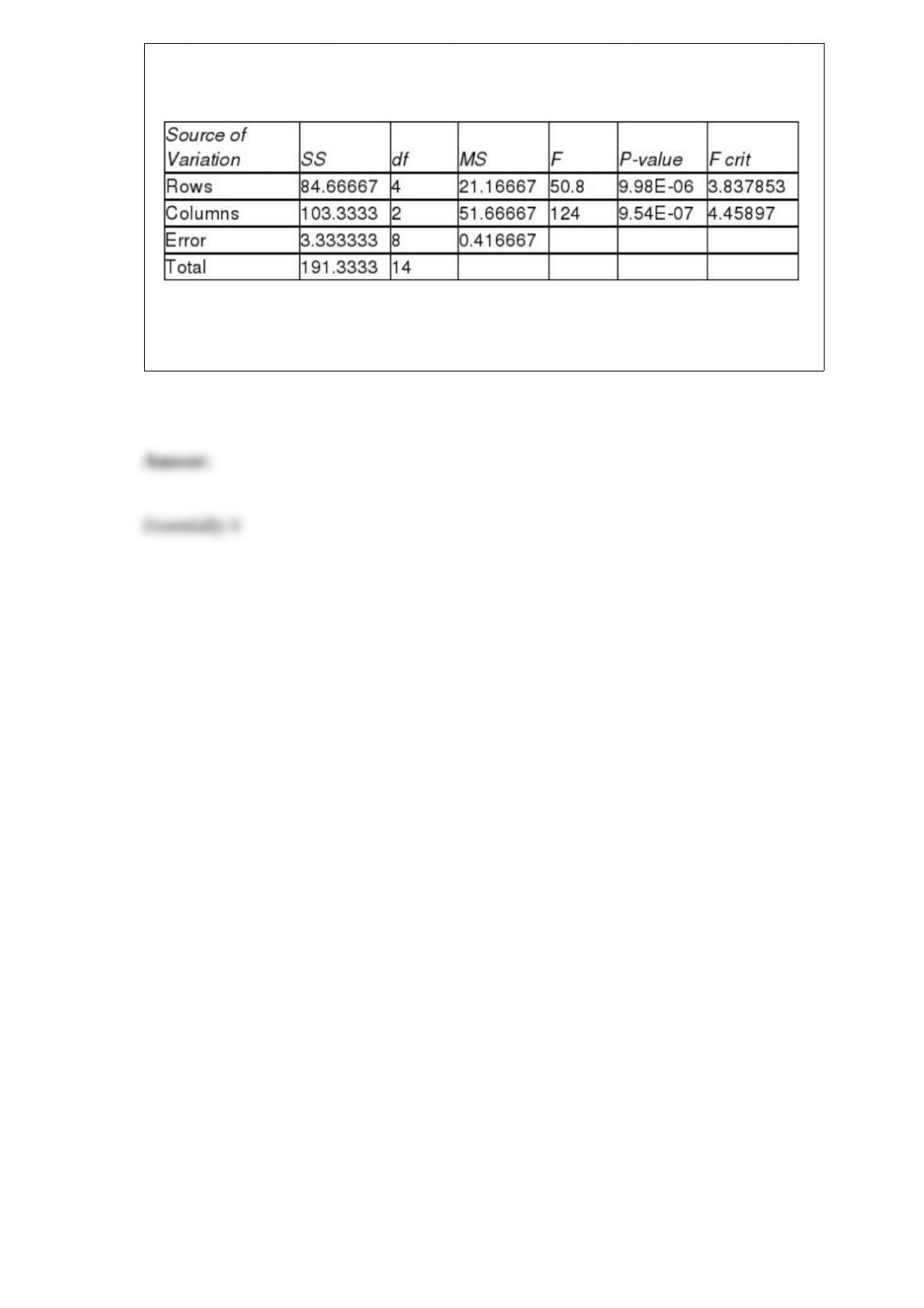
Below is the Excel output for the randomized block design:
Referring to Table 11-8, what is the p-value of the F test statistic for testing the block
effects?